X-Ray Light Curve of η Carinae from 3D SPH Simulations

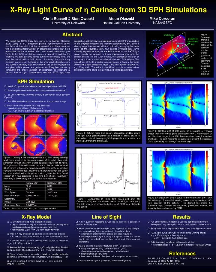
1. Figure 1: Cutaways showing relationship between the observer and the orbital geometry (pictured at apastron). Counter-clockwise is the prograde direction. orbital axis parallel to semi-major axis origin of X-ray emission We model the RXTE X-ray light curve for η Carinae (Corcoran 2005) using a 3-D smoothed particle hydrodynamics (SPH) simulation of the collision of the strong wind from the primary star with a weaker but faster wind of an assumed secondary star. For a reasonable choice of stellar, wind, and orbital parameters (see Table 1), the SPH simulations provide a dynamical model of the relatively low-density cavity carved out by the secondary wind, and how this varies with orbital phase. Assuming the main X-ray emission occurs near the head of the wind-wind interaction cone and varies in intensity with the inverse of the binary separation at any given orbital phase, we generate trial X-ray light curves by computing the phase variation of absorption to observers at various lines of sight. Comparisons with the RXTE light curve suggest an optimal viewing angle approximately 36o from apastron in the prograde direction and inclined approximately 54o. Such a viewing angle is consistent with the orbit being in roughly the same plane as the equatorial skirt. Our derived synthetic light curve naturally reproduces many of the key features of the RXTE light curve, namely the increase in X-rays approaching periastron, the sudden decline into the X-ray eclipse, the appropriate duration of the X-ray eclipse, and the less sharp incline out of the eclipse. The naturalness of the fit provides strong evidence in favor of the basic wind-wind binary interaction model, and with further analysis of, e.g., X-ray and UV spectra, it should be possible to place further constraints on the basic stellar, wind, and orbital parameters. observer i φ semi-major axis Figure 5: Contour plot of light curve as a function of viewing angles within the orbital plane (inclination i=90o). From bottom to top, the view ranges from 180o from apastron through apastron and back. The dark horizontal sequences represent the passage of the secondary star through the line of sight. Figure 3: Column mass (top panel), attenuation (middle panel), and light curve (bottom panel) as a function of orbital phase for the derived optimal viewing angle 36o prograde from apastron and inclined 54o from the orbital axis. Primary Star Secondary Star Mass 90 M 30 M Radius 90 R 30 R Wind Speed 500 km/s 3000 km/s Figure 6: Contour plot of light curve for fixed inclination of 54o and the full range of azimuthal viewing angles starting again at 180o from apastron at the bottom. The dashed line marks the azimuthal angle of φ=36o that is found to give closest match to the X-ray light curve observed by RXTE. Mass Loss Rate 2.5x10-4 M /yr 10-5 M /yr Figure 4: Comparison of RXTE data (black and gray; see Corcoran 2005) with the closest match model light curve (red). The light gray curve shows the first cycle of RXTE data shifted by one period. Eccentricity 0.9 Period 2.24 days Semi-major Axis 2.3x1014 cm X-Ray Light Curve of η Carinae from 3D SPH Simulations Mike Corcoran NASA/GSFC Chris Russell & Stan Owocki University of Delaware Atsuo Okazaki Hokkai-Gakuen University Abstract SPH Simulation • Need 3D dynamical model- cannot model periastron with 2D • Eulerian grid-based methods too computationally expensive • So use SPH code to model density & absorption in full 3D (see Figure 2) • But SPH method cannot resolve shocks that produce X-rays • So assume simple model for X-ray emission: • point-source at head of shock cone • Ix ~ 1/D, where D=Binary Separation Distance Figure 2: Density in the orbital plane for a 3D SPH binary colliding wind, from apastron to periastron (upper left to right), then post-periastron through recovery toward apastron (lower left to right). Through most of the orbit around apastron, the secondary’s wind (blue) carves out a nearly axisymmetric 2D cone in the denser but slower primary wind (red). But near and after periastron this cavity becomes embedded in the primary wind, giving rise to a "wind eclipse" of X-rays produced in the wind bow shock. Eventually this cavity is blown away and the conical form resumes. Table 1. Assumed stellar, wind, and orbital parameters. X-Ray Model Line of Sight Results • X-rays form in wind-wind interaction region • high-speed secondary wind slams into dense primary wind • ram balance depends on momentum ratio ≈4 • head located ≈ D/3 from secondary star • Model X-ray emission as point source near head of cone • To reduce noise, use 3/4 distance from secondary to head • Compute mass column density from source to observer, mo = (Figure 3, top) • Assume b-f absorption opacity x=5 cm2/g (Antokhin 2004) to compute X-ray attenuation exp(-x mo) (Figure 3, middle) • Since shock from secondary wind is nearly adiabatic, assume X-ray emission scales inversely with distance, Ix ~ 1/D • Derive resulting X-ray light curve as Lx ~ exp(-x mo)/D (Figure 3, bottom) • A key question regarding η Carinae is observer’s position in relation to binary orbit • Move observer to test how light curve depends on line of sight • φ: prograde angle from apastron in the orbital plane • i: inclination angle from the orbital axis (see Figure 1). • (A third possible angle, rotating the system about the line of sight, has no effect on the light curve and thus was not explored.) • Vary φ and i to match key features of RXTE light curve • steep rise approaching periastron (from Lx~1/D) • sharp drop near periastron (primary wind eclipse) • eclipse length of ~5% orbit • less steep climb out of eclipse (tail absorption vs. emission) • Optimal line of sight is φ=36o and i=54o (see Figure 4) • Full 3D dynamical model of η Carinae colliding wind density • compute X-ray absorption from source at head of shock cone • Study how line of sight affects light curve (see Figures 5 and 6) • RXTE light curve very well-fit, with optimal viewing angle: • φ = 36o -- prograde from apastron • i = 54o -- inclination from orbital axis • Orbit is roughly co-planar with equatorial skirt • inclination angle i = 54o vs. skirt inclination ~45o (Gull 2005) References Antokhin, I. I., Owocki, S. P., and Brown, J. C. 2004, ApJ, 611, 434 Corcoran, M. 2005, AJ 129, 2018 Gull, T. R. et al. 2005, BAAS 37, 1348