Download
1 / 55
570 likes | 881 Views
Partial Regression Plots. Life Insurance Example: (nknw364.sas). Y = the amount of life insurance for the 18 managers (in $1000) X 1 = average annual income (in $1000) X 2 = risk aversion score (0 – 10). Life Insurance: Input, diagnostics. title1 h = 3 'Insurance' ; data insurance;

E N D
Life Insurance Example: (nknw364.sas) Y = the amount of life insurance for the 18 managers (in $1000) X1 = average annual income (in $1000) X2 = risk aversion score (0 – 10)
Life Insurance: Input, diagnostics title1h=3'Insurance'; data insurance; infile'I:\My Documents\Stat 512\CH10TA01.DAT'; input income risk amount; run; procprintdata=insurance; run; *diagnostics; title2h=2'residual plots'; symbol1v=circle c=black; procregdata=insurance; model amount = income risk/rp; plotr.*(p. income risk); run;
Life Insurance: Scatter plot title2h=2'Scatterplot'; procsgscatterdata=insurance; matrix income risk amount; run;
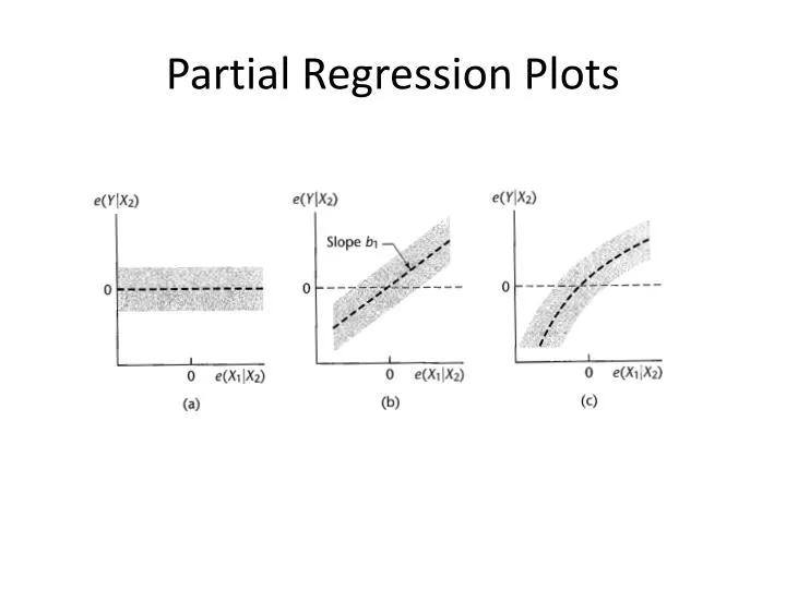
Life Insurance: Partial Regression Plots (1) procregdata=insurance; model amount=income risk/partial; run;
Life Insurance: Partial Regression Plots (2)risk title1h=3'Partial residual plot'; title2h=2'for risk'; symbol1v=circle i=rl; axis1label=(h=2'Risk Aversion Score'); axis2label=(h=2angle=90'Amount of Insurance'); procregdata=insurance; model amount risk = income; outputout=partialriskr=resamtresrisk; procgplotdata=partialrisk; plotresamt*resrisk / haxis=axis1 vaxis=axis2 vref = 0; run;
Life Insurance: Partial Regression Plots (2)income axis3label=(h=2'Income'); title2h=2'for income'; procregdata=insurance; model amount income = risk; outputout=partialincomer=resamtresinc; procgplotdata=partialincome; plotresamt*resinc / haxis=axis3 vaxis=axis2 vref = 0; run;
Life Insurance: Quadratic title1'Quadratic model'; title2''; data quad; set insurance; sinc = income; procstandarddata=quad out=quad mean=0; varsinc; data quad; set quad; incomesq = sinc*sinc; proccorrdata=quad; var amount risk income incomesq; run; procregdata=quad; model amount = income risk incomesq; run;
Life Insurance: normality Original Model With Quadratic Term
Life Insurance: Studentized Residuals (nknw364.sas) procregdata=quad; model amount=income risk incomesq/r; outputout = diagr=residstudent=student; run; procprintdata=diag; run;
Life Insurance: Studentized Deleted Residuals procregdata=quad; model amount=income risk incomesq/rinfluence; outputout = diag1 r=residrstudent=rstudent; run; procprintdata=diag1; run;
/r vs. /influence • /r keyword • /influence keyword
Life Insurance: Multicollinearity procregdata=quad; model amount=income risk incomesq/tolvif; run;
Body Fat: Multicollinearity (nknw260b.sas) databodyfat; infile'I:\My Documents\Stat 512\CH07TA01.DAT'; inputskinfold thigh midarm fat; procprintdata=bodyfat; run; procregdata=bodyfat; model fat=skinfold thigh midarm/viftol; run;
Blood Pressure Example: Background (nknw406.sas) Researching the relationship between blood pressure in healthy women ages 20 – 60. Y = diastolic blood pressure (diast) X = age n = 54
Blood Pressure: input data pressure; infile‘H:\My Documents\Stat 512\CH11TA01.DAT'; input age diast; procprintdata=pressure; run; title1h=3'Blood Pressure'; title2h=2'Scatter plot'; symbol1v=circle i=sm70 c=purple; axis1label=(h=2); axis2label=(h=2angle=90); procsortdata=pressure; by age; procgplotdata=pressure; plotdiast*age; run;
Blood Pressure: regression (unweighted) procregdata=pressure; modeldiast=age / clb; outputout=diagr=resid; run;
Blood Pressure: Residual Plots datadiag; setdiag; absr=abs(resid); sqrr=resid*resid; title2h=2'residual abs(resid) squared residual plots vs. age'; procgplotdata=diag; plot (residabsrsqrr)*age/haxis=axis1 vaxis=axis2; run;
Blood Pressure: computing weights procregdata=diag; modelabsr=age; outputout=findweightsp=shat; datafindweights; setfindweights; wt=1/(shat*shat);
Blood Pressure: computing weights if using resid2 proc reg data=diag; model sqrr=age; output out=findweights p=shat2; data findweights; set findweights; wt=1/shat2;
Blood Pressure: weighted regression procregdata=findweights; modeldiast=age / clbp; weight wt; outputout = weighted r = residp = predict; run;
Blood pressure: Comparison • Normal Regression • Weighted Regression
Blood Pressure: new residuals datagraphtest; set weighted; resid1 = sqrt(wt)*resid; title2h=2'Weighted data - residual plot'; symbol1v=circle i=nonecolor=red; procgplotdata=graphtest; plot resid1*predict/vref=0haxis=axis1 vaxis=axis2; run;
Body Fat Example (ridge.sas) n = 20 healthy female subjects ages of 25 – 34 Y = body fat (fat) X1 = triceps skinfoldthickness (skinfold) X2 = thigh circumference (thigh) X3 = midarmcircumference (midarm) Previous Conclusion: Problem with multicollinearity Good model with a) thigh only or with b) midarm and skinfold only
Body Fat Example: Regression (input) databodyfat; infile'I:\My Documents\Stat 512\CH07TA01.DAT'; inputskinfold thigh midarm fat; procprintdata=bodyfat; run; procregdata=bodyfat; model fat=skinfold thigh midarm; run;
Body Fat Example: Correlation proccorrdata=bodyfatnoprob;run;