Download
1 / 48
480 likes | 488 Views
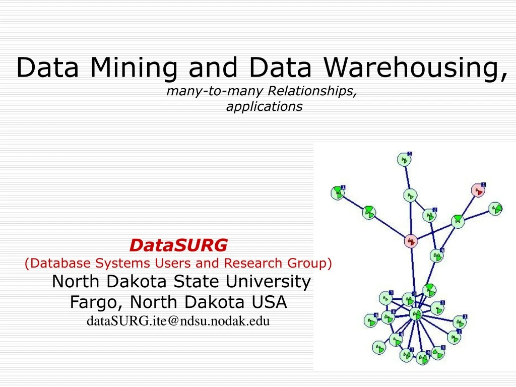
Data Mining and Data Warehousing, many-to-many Relationships, applications. DataSURG (Database Systems Users and Research Group) North Dakota State University Fargo, North Dakota USA dataSURG.ite@ndsu.nodak.edu.

E N D
Data Mining and Data Warehousing,many-to-many Relationships, applications DataSURG (Database Systems Users and Research Group) North Dakota State University Fargo, North Dakota USA dataSURG.ite@ndsu.nodak.edu
Data Mining on a Data Warehouse vs. Transaction Processing on a Data BaseWorkloadonRepository Question • C.J. Date, circa 1980 • Transactions on a DBMS vs. • file processing programs on file systems. • “Use a DBMS instead of file systems! Unify data resources, centralize control, promote standards and consistency, eliminate redundancy, increase data value and usage, yadda, yadda” • Circa 1990 • “Buy a separate DW for DM” (separate from your DBMS for TP)” • 2 separate, quite redundant, non-sharing, inconsistent.. systems! • What happened? • Great marketing success! (sold more hardware and software) • Great Concurrency Control R&D failure! We failed to integrate transactions and queries (OLTP and OLAP, i.e., updates and reads) in one system with acceptable performance! • The marketing was so successful, nobody noticed the failure!
OUTLINE I still hold out hope that DW and DB will eventually be unified again. I believe eventually the industry will demand it. Already, there’s work to update DWs! For now let’s just focus on DATA. • I Consider Data Mining (DM) to be on the unstructured side of querying. And on that side, you run up against two curses immediately. Curse of non-scalability(solutions don’t scale with data volume.) Curse of dimensionality(solutions don’t scale with data dimension • I will talk about techniques we use to address these curses. • Horizontal processing of vertically structured data (instead of the ubiquitous vertical processing of horizontal data (the record orientation). • Parallelize the DM engine. • Parallelize the software DM engine on clusters of computers. • Parallelize the greyware DM engine on clusters of people (i.e., browser-enable all software for visual data mining)
The DataSURG DM Architecture YOUR DATA data mining algorithms (yours/ ours) PREDICATE Count of objects satisfying PREDICATE Internet DMI (Data Mining Interface) DCI (Data Capture Interface) The Ptree Repository (lossless, compressed, vertically-structured replicas)
Data mining finds information in data.Why do we need Data Mining? • Data volume expands by Parkinson’s Law Data volume expands to fill available data storage • Disk-storage expands by Moore’s law Capacity 2 t / 9 months • Available storage doubles every 9 months!
We’re awash with data! • Network data: hi-speed, DWDM, All-opt(mgmt, flow classif’n,QoS,security) (10 terabytes by 2003 ~ 1013 B). • US EROS Data Center (EDC) archives Earth Observing System (EOS) Remotely Sensed Imagery (RSI), satellite and aerial photo data (10 petabytes by 2005 ~ 1016 B). • National Virtual Observatory (aggregated astronomical data) (10 exabytes by 2010 ~ 1019 B). • Sensor data from sensors (including Micro & Nano -sensor networks) (10 zettabytes by 2015 ~ 1022 B). • WWW (and other text collections) (10 yottabytes by 2020 ~ 1025 B). • Genomic/Proteomic/Metabolomic data(microarrays, genechips, genome sequences) (10 gazillabytes by 2030 ~ 1028 B?). • Stock Market prediction data (prices + all the above? especially astronomy data?) (10 supragazillabytes by 2040 ~ 1031 B?). Useful information must be teased out of these large volumes of data through data mining. I had to make up this Name! Projected data sizes are overrunning our ability to name those sizes!
More’s Law: More’s Less The more volume, the less information.(AKA: Shannon’s Canon) A simple illustration: Which phone book has more info? (both involve the same 4 data granules) BOOK-1BOOK-2 Name NumberName Number Smith 234-9816 Smith 234-9816 Jones 231-7237 Smith 231-7237 Jones 234-9816 Jones 231-7237 Data mining reduces volume and raises the information level.
TIFF image Yield Map Precision Agriculture Data Mining Dataset consists of an aerial photograph (TIFF image taken during the growing season) and a synchronized yield map (crop yield taken at harvest). Altogether there are 4 feature attributes (B,G,R,Y) and ~100,000 pixels. A producer wants to know the relationship between the color intensities and yield? One hypothsize, the Association Rule, hi_greenandlow_red hi_yield, is intuitive and could be made and verified without data mining (simple querying). Data mining has found a stronger rule, hi_NIR and low_red very_hi_yield. So many producers use VIR instead of RBG cameras to get the better information.
Another Precision Agriculture Data Mining Example: Grasshopper Infestation Prediction(again involving RSI data) • Grasshopper caused significant economic loss each year. • Early infestation prediction is key to damage control. Pixel classification on remotely sensed imagery holds significant promise to achieve early detection. Pixel classification (signaturing) has many applications pest detection, forest fire detection, wet-lands monitoring … (for signaturing we developed the SMILEY software/greyware system) http:midas.cs.ndsu.nodak.edu/~smiley
Sensor Network Data Mining • Micro and Nano scale sensor blocks are being developed for sensing • Biological agents • Chemical agents • Motion detection • coatings deterioration • RF-tagging of inventory • Structural materials fatigue • There will be trillions++ of individual sensors creating mountains of data. • The data must be mined for it’s information.
Situation space (with nano-sensors ) Sensor Network Application: CubE for Active Situation Replication (CEASR) Operational Capability: Using Alien Technology’s Fluidic Self-assembly (FSA) technology, clear layers (with embedded nano-LED elements) laminated together produce a visualization cube (a nano-LED at each pixel corresponding to a nano-sensors at each pixel in the situation space. Nano-sensors turn on CEASR display Nano-LEDs when a threshold level (chemical, vibrational, biological, thermal…) is exceeded.. • Proposed Technical Approach: • Sense chemical, vibrational, biological, thermal in real-time. • The problems to be solved include: • Communication between sensor field(s) and CEASR. • Nano-sensors position registration. • Fluidic Self Assembly (FSA) of Cube. • FSA is an Alien Technology patented process capable of producing clear flexible substrates with embedded nano-LED display units. Each energized nano-sensor must transmit a ping together with its location. These locations are then translated to 3-dimensional coordinates at the display. The corresponding voxel on the display lights up. A more sophisticated CEASR device would sense and transmit the intensity levels, lighting up the display voxel with the same intensity.
Anthropology ApplicationDigital Archive Network for Anthropology (DANA)(data mine arthropological artifacts (shape, color, discovery location,…)
dec RA Astronomy Application: The celestial sphere
Data Mining? Querying is asking specific questions and expecting specific answers. Data Miningis going into the MOUNTAIN of DATA, and returning with information gems. But also, some fool’s gold? Relevance and interestingness analysis, serves to assay those information and knowledge gems.
Data Mining Process Pattern Evaluation and Assay • Data mining: the core of the knowledge discovery process. Data Mining OLAP Classification Clustering ARM Task-relevant Data Data Warehouse: cleaned, integrated, read-only, periodic, historical raw database Selection Feature extraction, tuple selection Data Cleaning/Integration: missing data, outliers, noise, errors Mountain of Raw Data
Fractals, … Standard querying Searching and Aggregating Data Prospecting Machine Learning Data Mining Association Rule Mining OLAP (rollup, drilldown, slice/dice.. Supervised Learning – classification regression SQL SELECT FROM WHERE Complex queries (nested, EXISTS..) FUZZY query, Search engines, BLAST searches Unsupervised Learning - clustering Data Mining versus Querying There is a whole spectrum of techniques to get information from data: On the Query end, much work is yet to be done(D. DeWitt, ACM SIGMOD Record’02). On the Data Mining end, the surface has barely beenscratched. But even those scratches had a great impact – One of the early scatchers became the biggest corporation in the world last year. A Non-scratcher filed for bankruptcy Walmart vs.KMart
Our Approach • Vertical, compressed data structures, variously called either Predicate-trees or Peano-trees (Ptrees in either case)1 processed horizontally(DBMSs processhorizontal data vertically) • Ptrees are data-mining-ready, compressed data structures, which attempt to address the curses of scalability and curse of dimensionality. • A compressed, OLAP-ready data warehouse structure, the Pcube1 which facilitate OLAP and querying, using Ptrees. 1 Technology is patent pending by North Dakota State University
A table, R(A1..An), is a horizontal structure (set of horizontal records) Ptrees vertical partition; compress each vertical bit slice into a basic Ptree; R( A1 A2 A3 A4) -->R[A1] R[A2] R[A3] R[A4] 010 111 110 001 011 111 110 000 010 110 101 001 010 111 101 111 101 010 001 100 010 010 001 101 111 000 001 100 111 000 001 100 010 111 110 001 011 111 110 000 010 110 101 001 010 111 101 111 101 010 001 100 010 010 001 101 111 000 001 100 111 000 001 100 Horizontal structure Processed vertically (scans) 0 0 0 0 1 0 1 1 R11 R12 R13 R21 R22 R23 R31 R32 R33 R41 R42 R43 0 1 0 1 1 1 1 1 0 0 0 1 0 1 1 1 1 1 1 1 0 0 0 0 0 1 0 1 1 0 1 0 1 0 0 1 0 1 0 1 1 1 1 0 1 1 1 1 1 0 1 0 1 0 0 0 1 1 0 0 0 1 0 0 1 0 0 0 1 1 0 1 1 1 1 0 0 0 0 0 1 1 0 0 1 1 1 0 0 0 0 0 1 1 0 0 0 0 0 1 0 01 0 1 0 1 0 0 1 0 0 1 01 1. Whole file is not pure1 0 2. 1st half is not pure1 0 0 0 0 0 1 01 P11 P12 P13 P21 P22 P23 P31 P32 P33 P41 P42 P43 3. 2nd half is not pure1 0 0 0 0 0 1 0 0 10 01 0 0 0 1 0 0 0 0 0 0 0 1 01 10 0 0 0 0 1 10 0 0 0 0 0 0 0 1 0 0 0 0 0 0 0 0 0 0 1 1 0 0 0 0 1 10 0 1 0 0 0 0 1 0 1 4. 1st half of 2nd half not 0 0 0 1 0 1 01 5. 2nd half of 2nd half is 1 0 1 0 6. 1st half of 1st of 2nd is 1 Eg, to count, 111 000 001 100s, use “pure111000001100”: 0 23-level P11^P12^P13^P’21^P’22^P’23^P’31^P’32^P33^P41^P’42^P’43 = 0 0 22-level=2 01 21-level 7. 2nd half of 1st of 2nd not 0 horizontally process these Ptrees using one multi-operand logical AND operation. processed vertically (vertical scans) 1-Dimensional Ptrees are built by recording the truth of the predicate “pure 1” recursively on halves, until there is purity, P11:
Horizontal Processing of Vertical StructuresHistory • In the 1980’s vertical data structures were proposed for record-based workloads • Decomposition Storage Model (DSM, Copeland et al) • Attribute Transposed File (ATF) • Band Sequential (BSQ) in RSI) • Bit Transposed File (BTF, Wang et al) • These initiatives didn’t last. Why not?
R( A1 A2 A3 A4) 010 111 110 001 011 111 110 000 010 110 101 001 010 111 101 111 101 010 001 100 010 010 001 101 111 000 001 100 111 000 001 100 R11 R12 R13 R21 R22 R23 R31 R32 R33 R41 R42 R43 R11 R12 R13 R21 R22 R23 R31 R32 R33 R41 R42 R43 0 1 0 1 1 1 1 1 0 0 0 1 0 1 1 1 1 1 1 1 0 0 0 0 0 1 0 1 1 0 1 0 1 0 0 1 0 1 0 1 1 1 1 0 1 1 1 1 1 0 1 0 1 0 0 0 1 1 0 0 0 1 0 0 1 0 0 0 1 1 0 1 1 1 1 0 0 0 0 0 1 1 0 0 1 1 1 0 0 0 0 0 1 1 0 0 0 1 0 1 1 1 1 1 0 0 0 1 0 1 1 1 1 1 1 1 0 0 0 0 0 1 0 1 1 0 1 0 1 0 0 1 0 1 0 1 1 1 1 0 1 1 1 1 1 0 1 0 1 0 0 0 1 1 0 0 0 1 0 0 1 0 0 0 1 1 0 1 1 1 1 0 0 0 0 0 1 1 0 0 1 1 1 0 0 0 0 0 1 1 0 0 Horizontal Processing of Vertical Structuresfor Record-based Workloads • For record-based workloads (where the result is a set of records), changing the horizontal record structure and then having to reconstruct it, may have introduced too much post processing? • For data mining workloads, the result is often a bit (Yes/No, True/False) or another unstructured result, there is no reconstructive post processing? 1
Run Lists: Generalized Ptrees using standard run length compression of vertical bit files (alternatively, using Lempl Zipf?, Golomb?, other?) R( A1 A2 A3 A4) -->R[A1] R[A2] R[A3] R[A4] 010 111 110 001 011 111 110 000 010 110 101 001 010 111 101 111 101 010 001 100 010 010 001 101 111 000 001 100 111 000 001 100 010 111 110 001 011 111 110 000 010 110 101 001 010 111 101 111 101 010 001 100 010 010 001 101 111 000 001 100 111 000 001 100 R11 0 0 0 0 1 0 1 1 • 1st run is Pure0 0:000 • truth:start R11 R12 R13 R21 R22 R23 R31 R32 R33 R41 R42 R43 0 1 0 1 1 1 1 1 0 0 0 1 0 1 1 1 1 1 1 1 0 0 0 0 0 1 0 1 1 0 1 0 1 0 0 1 0 1 0 1 1 1 1 0 1 1 1 1 1 0 1 0 1 0 0 0 1 1 0 0 0 1 0 0 1 0 0 0 1 1 0 1 1 1 1 0 0 0 0 0 1 1 0 0 1 1 1 0 0 0 0 0 1 1 0 0 2. 2nd run is Pure1 1:100 3.3rd run is Pure0 0:101 4. 4th run is Pure1 1:110 RL11 RL12 RL13 RL21 RL22 RL23 RL31 RL32 RL33 RL41 RL42 RL43 0:000 1:010 0:101 1:000 0:001 1:010 0:100 1:101 0:110 1:000 0:100 1:000 0:110 1:000 0:010 1:011 0:100 1:000 0:100 1:000 0:010 0:000 1:010 0:000 1:010 0:000 1:001 0:010 1:100 0:101 1:110 0:000 1:100 0:101 1:110 1:000 0:100 1:101 Eg, to count, 111 000 001 100s, use “pure111000001100”: RL11^RL12^RL13^RL’21^RL’22^RL’23^RL’31^RL’32^RL33^RL41^RL’42^RL’43 Run Lists: record type and start-offset of pure runs. E.g., RL11: RL11 0:000 1:100 0:101 1:110 (to complement, flip purity bits)
R11 0 0 0 0 1 0 1 1 RL110:000 1:100 0:101 1:110 1. Whole file is not pure1 0 2. 1st half is not pure1 0 3. 2nd half is not pure1 0 0 0 0 0 1 1 0 0 0 0 0 0 0 0 1 10 0 0 0 0 1 0 0 0 0 0 0 4. 1st half of 2nd half not 0 5. 2nd half of 2nd half is 1 6. 1st half of 1st of 2nd is 1 7. 2nd half of 1st of 2nd not 0 RunList-trees? (RLtrees) • To facilitate subsetting (isolating a subset) and processing, a Ptree stucture can be constructed on top of the RunList using the “pure1” predicate:
R11 0 0 0 0 1 0 1 1 RL110:000 1:100 0:101 1:110 1. Whole file is true 1 2. 1st half is false 0 3. 2nd half is true 1 1 0 1 1 1 1 1 0 1 1 1 0 1 1 1 10 1 0 1 1 1 1 0 1 1 0 1 4. 1st half of 2nd half true 1 5. 2nd half of 2nd half true 1 6. 1st half of 1st of 2nd true 1 7. 2nd of 1st of 2nd false 0 RunList-trees continued • Alternatively, a separate NotPure0 index trees could be build where the predicate is NotPure0 (also note, the tree could be terminated at a given level). • First, AND the NP0 index trees. • Only the 1-branches or the resulty need to be ANDed through list scans. • The more operands, the fewer 1-branches.
Ptrees Vertical, compressed, lossless structures that facilitates fast horizontal AND-processing • The jury is still out on the best parallelization approach, vertical (by relation) or horizontal (by tree node) or some combination. • Horizontal parallelization is pretty, but network multicast overhead is huge • Use active networking? Clusters of Playstations?... • The most useful form of a Ptree is the Pure1-tree or P1tree • A 1-bit at a node iff corresponding half is pure1. • There are many other useful predicates, e.g., NonPure0-trees • But we will focus on P1trees. • All Ptrees shown so far were • 1-dimensional (recursively halving bit files),but they can be • 2-D (recursively quartering) (e.g., used for 2-D images) • 3-D (recursively eight-ing), …
0 0 1 1 1 1 1 1 0 0 1 1 1 1 1 0 0 0 1 1 1 1 1 1 0 0 1 1 1 1 1 1 1 0 1 1 1 1 0 0 0 0 1 1 1 1 0 0 0 0 1 1 1 1 0 0 0 0 0 1 1 1 0 0 0 0 1 1 0 0 0 0 0 0 0 0 0 0 1 1 0 0 1 1 1 1 0 0 1 1 1 1 1 1 1 1 0 0 0 0 0 0 1 1 0 0 1 1 1 1 0 0 1 1 A 2-Dimensional P1tree Node is 1 iff that quadrant is purely 1-bits, e.g., A bit-file(from, e.g., a 2-D image) 1111110011111000111111001111111011110000111100001111000001110000 Run-length compress the corresponding raster ordered matrix using Peano order.
001 55 level-3 (pure=43) 1 1 1 1 1 1 0 0 1 1 1 1 1 0 0 0 1 1 1 1 1 1 0 0 1 1 1 1 1 1 1 0 1 1 1 1 1 1 1 1 1 1 1 1 1 1 1 1 1 1 1 1 1 1 1 1 0 1 1 1 1 1 1 1 0 1 2 3 16 8 15 16 level-2 2 3 0 4 1 4 4 3 4 level-1 3 111 1 1 1 0 0 0 1 0 1 1 0 1 level-0 2 . 2 . 3 ( 7, 1 ) 10.10.11 ( 111, 001 ) Alternatively, a Count tree?Counts are the ultimate goal, but P1trees are more compressed and produce the needed counts quite quickly. • QID (Quadrant ID): e.g., 2.2.3 • Pure-1/Pure-0 quadrants • Root Count • Tree levels: 3, 2, 1, 0 (purity counts of 43 42 41 40 resp.) • Fan-out = 2dim = 4
Logical Operations on Ptrees(are used to get counts of any pattern) AND operation is faster than the bit-by-bit AND since, there are shortcuts (any pure0 operand node means result node is pure0.) e.g., only load quadrant 2 to AND Ptree1, Ptree2, etc. The more operands there are in the AND, the greater the benefit due to this shortcut (more pure0 nodes). Ptree 1 Ptree 2 AND result OR result
Situation space (with nano-sensors ) A Natural 3-D Application: CubE for Active Situation Replication (CEASR) Operational Capability: Using Alien Technology’s Fluidic Self-assembly (FSA) technology, clear layers (with embedded nano-LED elements) laminated together produce a visualization cube (a nano-LED at each pixel corresponding to a nano-sensors at each pixel in the situation space. Nano-sensors turn on CEASR display Nano-LEDs when a threshold level (chemical, vibrational, biological, thermal…) is exceeded.. • Proposed Technical Approach: • Sense chemical, vibrational, biological, thermal in real-time. • The problems to be solved include: • Communication between sensor field(s) and CEASR. • Nano-sensors position registration. • Fluidic Self Assembly (FSA) of Cube. • FSA is an Alien Technology patented process capable of producing clear flexible substrates with embedded nano-LED display units. Each energized nano-sensor must transmit a ping together with its location. These locations are then translated to 3-dimensional coordinates at the display. The corresponding voxel on the display lights up. A more sophisticated CEASR device would sense and transmit the intensity levels, lighting up the display voxel with the same intensity.
Another Natural 3-D ApplicationDigital Archive Network for Anthropology (DANA)(data mine arthropological artifacts (shape, color,…)
3-Dimensional Ptrees (e.g., for the CEASR sensor network or the Digital Archive Network for Anthropology)
Ptree dimension • The dimension of the Ptree structure is a user chosen parameter • It can be chosen to fit the data dimension • Most datasets 1-D Ptrees (recursive halving) • 2-D Images 2-D Ptrees (recursive quartering) • 3-D Solids 3-D Ptrees (recursive eighth-ing) • Or dimension can be chosen based on other considerations • optimize compression • increase processing speed (next slide)
Raster Sorting: Attributes 1st Bit position 2nd Peano Sorting: Bit position 1st Attributes 2nd Generalized Raster and Peano Sorting: generalizes to any table with numeric attributes (not just images).
KNN speed improvement (UCI MLR data sets) 120 Unsorted 100 80 Time in Seconds Generalized Raster 60 40 Generalized Peano 20 0 crop adult spam function mushroom Generalize Peano Sorting
National Virtual Observatory data • What Ptree dimension and what ordering should be used for astronomical data? • Where all bodies are assumed to be on the surface of a sphere, the celestial sphere (shares equatorial plane with earth and has no specified radius) • Peano Triangle Mesh Tree (PTM-tree) • Peano Celestial Coordinate tree (PCCtree) • Uses (RA, dec) coordinates of the celestial sphere • RA=Recession Angle (longitudinal angle) • dec=declination (latitude angle)
Peano Triangular Mesh Tree (PTM-tree) • Similar to the Hierarchical Triangular Mesh (HTM) used in the Sloan Digital Sky Survey project. In both: • Sphere is divided into triangles • Triangle sides are always great circle segments. • PTM differs from HTM in the way in which they are ordered?
1 1 1,2 1,2 1,1,2 1,3,3 1,0 1,3,0 1,0 1,1,1 1,3,2 1,3 1,1,0 1,1 1,3,1 1.1.3 1,1 1,3 The difference between HTM and PTM-trees is in the ordering. Ordering of PTM-tree Ordering of HTM Why use a different ordering?
dec RA PTM Triangulation of the Celestial Sphere Traverse southern hemisphere in the revere direction (just the identical pattern pushed down instead of pulled up, arriving at the Southern neighbor of the start point. This “Peano ordering” produces a sphere-surface filling curve with good continuity characteristics.
PTM triangulation – Next Level LRLR LRLR LRLR LRLR
PTM-triangulation - Next Level LRLR RLRL LRLR RLRL LRLR RLRL LRLR RLRL LRLR RLRL LRLR RLRL LRLR RLRL LRLR RLRL
Peano Celestial Coordinate Trees (PCCtrees) • Unlike PTM-trees which initially partition the sphere into the 8 faces of an octahedron, in the PCCtree scheme: • the sphere is tranformed into a cylinder, • then into a rectangle, • then standard Peano ordering is used on the Celestial Coordinates. • Celestial Coordinates • RA is from 0 to 360o • dec is -90o to 90o.
PRAd e c 90o 0o -90o Z Z Z Z Z Z Z Z Z Z Z Z Z Z Z Z Z Z Z Z Z Z Z Z Z Z Z Z Z Z Z Z Z Z Z Z Z Z Z Z Z Z Z Z Z Z Z Z Z Z Z Z Z Z Z Z Z Z Z Z Z Z Z Z Z Z Z Z Z Z Z Z Z Z Z Z Z Z Z Z Z Z Z Z Z Z Z Z Z Z Z Z Z Z Z Z Z Z Z Z Z Z Z Z Z Z Z Z Z Z Z Z Z Z Z Z Z Z Z Z Z Z Z Z Z Z Z Z Z Z Z Z Z Z Z Z Z Z Z Z Z Z Z Z Z Z Z Z Z Z Z Z Z Z Z Z Z Z Z Z Z Z Z Z Z Z Z Z Z Z Z Z Z Z Z Z Z Z Z Z Z Z Z Z Z Z Z Z Z Z Z Z Z Z Z Z Z Z Z Z Z Z Z Z Z Z Z Z Z Z Z Z Z Z Z Z Z Z Z Z Z Z Z Z Z Z Z Z Z Z Z Z Z Z Z Z Z Z Z Z Z Z Z Z Z Z Z Z Z Z Z Z Z Z Z Z 0o 360o North Plane Z Z Z Z Z Z Z Z Z Z Z Z Z Z Z Z Z Z Z Z Z Z Z Z Z Z Z Z Z Z Z Z Z Z Z Z Z Z Z Z Z Z Z Z Z Z Z Z Z Z Z Z Z Z Z Z Z Z Z Z Z Z Z Z Z Z Z Z Z Z Z Z Z Z Z Z Z Z Z Z Z Z Z Z Z Z Z Z Z Z Z Z Z Z Z Z Z Z Z Z Z Z Z Z Z Z Z Z Z Z Z Z Z Z Z Z Z Z Z Z Z Z Z Z Z Z Z Z Z Z Z Z Z Z Z Z Z Z Z Z Z Z Z Z Z Z Z Z Z Z Z Z Z Z Z Z Z Z Z Z Z Z Z Z Z Z Z Z Z Z Z Z Z Z Z Z Z Z Z Z Z Z Z Z Z Z Z Z Z Z Z Z Z Z Z Z Z Z Z Z Z Z Z Z Z Z Z Z Z Z Z Z Z Z Z Z Z Z Z Z Z Z Z Z Z Z Z Z Z Z Z Z Z Z Z Z Z Z Z Z Z Z Z Z Z Z Z Z Z Z Z Z Z Z Z Z South Plane PRAdec-scheme: Sphere Cylinder Plane
Graph data(many-to-many self relations) “Everything should be made as simple as possible, but not simpler” Albert Einstein
Representating graphs Examples: • Genomics • Protein-protein interactions (ACM KDD-Cup ’02) • Focuses is on node structure • WWW • Focuses on link structure • Publications citations • ACM KDD_Cup ’03 • Focus is on both Scientific American 05/03
SubCell-Location Myta Ribo Nucl Ribo 17, 78 12, 60 Mi, 40 1, 48 10, 75 0 0 7, 40 0 14, 65 0 0 16, 76 0 9, 45 Pl, 43 Function apop meio mito apop StopCodonDensity .1 .1 .1 .9 PolyA-Tail 1 1 0 0 Organism Species Vert Genome Size (million bp) Gene Dimension Table g0 g1 g2 g3 o0 human Homo sapiens 1 3000 Organism Dimension Table o1 fly Drosophila melanogaster 0 185 o2 1 1 1 1 1 0 0 1 0 1 0 0 1 0 1 1 o3 0 1 0 1 1 0 0 1 0 1 0 1 1 0 0 0 yeast Saccharomyces cerevisiae 0 12.1 e0 1 0 1 1 0 1 1 1 1 1 0 1 1 0 1 0 e0 mouse Mus musculus 1 3000 e1 e1 e2 e2 e3 LAB PI UNV STR CTY STZ ED AD S H M N e3 Experiment Dimension Table (MIAME) 3 2 a c h 1 2 2 b s h 0 2 4 a c a 1 2 4 a s a 1 Genomics Gene-OrgDim Tablechromosome,length Gene-Experiment-Organism Cube (1 iff that gene from that organism expresses at a threshold level in that experiment.) Many-to-many-to-many relationship
Protien-Protien Interactions (PPI) (2-hop interactions) SubCell-Location Myta Ribo Nucl Ribo g0 g0 1 0 0 1 g1 Myta Ribo Nuc l apop Me i o Mi to SCD 1 SCD 2 SCD 3 SCD 4 Poly-A G E N E 0 1 1 g2 0 1 0 1 g3 1 0 g1 0 1 1 0 1 1 0 0 1 0 1 0 0 0 1 1 g1 0 1 0 1 g2 1 0 0 0 1 0 0 1 0 0 0 0 1 1 g2 0 1 0 0 g3 0 0 1 0 0 1 0 0 0 1 0 g3 0 1 0 1 0 0 1 0 0 1 0 g4 Gene Dimension Table (Binary) g3 g2 g1 g0 Function apop meio mito apop StopCodonDensity .1 .1 .1 .9 Gene Dimension Table PolyA-Tail 1 1 0 0 0
Myta Ribo Nuc l apop Me i o Mi to SCD length essential Dis-center Info-qty G E N E 1 0 0 1 0 1 o 4 1 1 4 g1 0 1 0 0 1 0 .1 6 0 5 1 g2 0 0 1 0 0 1 .1 4 0 0 5 g3 0 1 0 1 0 0 .9 9 0 8 2 g4 Gene Dimension Table (non-binary) Greyware PPI graph mining tool • Visualize feature information using a glyph for each gene (PPI graph node) • PPI Edge iff the 2 genes code for interacting proteins This visual data mining tool was effective in KDD-CUP ’02) Glyph for g1 stopcodondensity
Thanks so much! • Don’t forget to submit your best work to CAINE, Nov 11-13, 2003, Las Vegas NV by July 1. Submit to Program Chair, kendall.nygard@ndsu.nodak.edu or Conference Chair, william.perrizo@ndsu.nodak.edu http:/www.cs.ndsu.nodak.edu/~krile/caine03 or http:www.isca-hq.org For those interested in DM in genomics and bioinformatics, Virtual Conference in Genomics and Bioinformatics VGAB-III, Sep 16-18, 2003http:www.ndsu.edu/~virtual-genomicsSubmit papers toProgram Chair, willy.valdivia@ndsu.nodak.edu or to the Conference Chair, william.perrizo@ndsu.nodak.edu • VGAB-III will be available over Access Grid and Real Player to anywhere, for free (no registration fee)