Download
1 / 31
310 likes | 502 Views
Linear Prediction Filters and Neural Networks. Paul O’Brien ESS 265, UCLA February 8, 1999. Outline. Neural Networks Uses System Description Time Evolution Theory Training Network Analysis Examples Dst- D H Dst-VBs. Linear Prediction Filters Uses System Description

E N D
Linear Prediction Filters and Neural Networks Paul O’Brien ESS 265, UCLA February 8, 1999
Outline • Neural Networks • Uses • System Description • Time Evolution • Theory • Training • Network Analysis • Examples • Dst-DH • Dst-VBs • Linear Prediction Filters • Uses • System Description • Time Evolution • Green’s Functions • Construction • Filter Analysis • Examples • Dst-DH • Dst-VBs
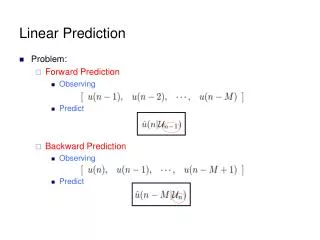
Linear Prediction Filter Uses • Map one Input (or many) to one Output • Convert Dst to Single Ground-station DH • Make a Forecast • Convert Solar Wind Measurements To Geomagnetic Indices • Determine System Dynamics • Use Impulse Response To Determine Underlying Ordinary Differential Equation
AR MA What an LPF Looks Like • An LPF can have an autoregressive (AR) part and a moving average (MA) part • AR part describes internal dynamics • MA part describes external dynamics • Ambiguity occurs when used separately
Other Names for LPFs • Convolution Filter • Moving Average • Infinite Impulse Response Filter (IIR) • Finite Impulse Response Filter (FIR) • Recursive Filter • ARMA Filter • LPFs are a subset of Linear Filters which relate the Fourier spectra of two signals
MA Filters Are Green’s Functions • Ordinary Differential Equations Can Be Solved with Greens Functions:
AR Filters Are Differential Equations • Ordinary Differential Equations Can Be Rewritten As AR Filters:
Determining LPF Coefficients The a’s and b’s are found by solving an overdetermined matrix equation: Often tk = t0+kDt Solved using Least Squared Error Optimization or Singular Value Decomposition
More on Linear Filters • The Linear Filter formalism can be extended to multiple inputs • There is an ambiguity between the MA and AR parts for certain kinds of differential equations. An ARMA filter can greatly simplify some MA filters
Handling Data Gaps • Missing Inputs • Omit intervals with data gaps, if possible • Interpolation over data gaps will smear out MA coefficients • Missing Outputs • Omit intervals with data gaps • Interpolation over data gaps can ruin the AR coefficients • Less sensitive to interpolation in lag outputs
Exponential Decay bj bj Recurrence lag lag Derivative Operator bj lag Linear Filter Analysis • Once the filter coefficients are determined, we relate them to ODEs
LPF Localization • Localization adds Nonlinearity • Nonlocal LPFs cannot handle nonlinear dynamics • Localize in Time • Continuously reconstruct LPF based only on most recent data • Can be very accurate but hard to interpret • Localize in State Space • Construct different LPF for each region of state space • Can provide multivariate nonlinearity
LPF Example: Dst-DH • Dst is a weighted average of DH measured at 4 stations around the globe. • Depending on activity and the local time of a station, there is a different relationship between Dst and DH • We will localize this filter in 24 1-hour bins of local time • The filter will be very simple: DH(t) = b0(lt) Dst(t) • lt is the local time of the station at time t • We solve this equation in each 1-hour bin of local time • By plotting b0 vs lt, we can infer the local current systems • This local current system is believed to be the partial ring current
Partial Ring Current DHSJG-Dst 1-Point Filter by Local Time • Localized Filter: DH = b0(lt)Dst • Dst is less intense than DH near Dusk due to an enhanced Ring Current in the Dusk sector 1.2 1 1/b0 0.8 Local Dusk 0.6 0 4 8 12 16 20 24 Local Time
LPF Example: Dst-VBs • The Ring Current (Dst) is largely driven by the solar wind • One good “coupling function” for the solar wind driver is the interplanetary electric field (VBs) • We construct a long MA filter:
4 3 2 bj 1 0 -1 -5 0 5 10 15 20 25 30 35 40 45 Lag (hours) Dst-VBs Filter Coefficients • Note the roughly exponential decay • The differential equation could be: • We can, therefore, build a trivial ARMA filter to do the same job:
Neural Network Uses • Map multiple Inputs to one Output (or many) • Excellent nonlinear interpolation but not reliable for extrapolation • Make a forecast • Excellent for forecasting complex phenomena • Determine System Dynamics • NN is a black box model of the system • Run NN on simulated data to isolate system response to individual inputs • Many exotic NNs exist to perform other tasks
NN Theory • Based on biological neural systems • Biological NN: composed of connections between individual neurons • Artificial NN: composed of weights between perceptrons • We don’t know exactly how biological neural systems learn, so we have made some approximate training schemes • Artificial NNs excel at quantifying • Biological NNs excel at qualifying
h1 I1 h2 I2 O1 h3 I3 h4 NN Topology • A standard Feed Forward NN has no recursive connections • Arrows represent weights (w,v) and biases (b,c) • hi and Oi are perceptrons • Typically only one hidden layer is necessary • More hidden units allow for more complexity in fitting (not always good) • Nonlinearity is achieved through an activation function • tanh(x) or [1+e-x]-1 wi nij • This is equivalent to an MA Filter • AR behavior can be achieved through recurrence
h1 h1 I1 I1 h2 h2 I2 wi O1 I2 wi O1 h3 h3 I*3 nij I*3 h4 nij h4 NN Recurrence • An Output Recurrent network is useful when O(t) depends on O(t-Dt) • The recurrence is usually only implicit during training: I*3 is taken from actual data rather than previous O1 Pseudo-Input Pseudo-Input • An Elman Network is useful when O(t) depends on the time history of the Inputs • This makes training rather difficult • Continuous time series are needed • Batch optimization is impossible
NN Training Theory • A NN is initialized with a random set of weights • It is trained to find the optimal weights • Iteratively adjust the weights • Target least squared error for most data • Target relative error for data with rare large events • There must be far more training samples than there are weights • At least a factor of 10 • The goal is to achieve a fit which will work well out of sample as well as in sample • Poor out of sample performance is a result of overfitting
Gradient Descent NN Output • Simplest non-linear optimization • Weights are corrected in steps down the error gradient • A learning rateh is used to ensure smooth convergence to error minimum • Descent can be stabilized by adding momentum m, which recalls DW(s-1) from last step • m and h should be between 0 and 1, sometimes functions of s • For recurrent networks, gradient descent should be done serially for each tk • This type of Gradient Descent replaces Backpropagation W is a vector holding all the NN weights and biases
Levenberg-Marquardt Training • LM training is much faster than gradient descent • LM training is not very appropriate for recurrent networks • Algorithm: 1. Increase m until a step can be taken without increasing the error 2. Decrease m while error decreases with each step 3. Repeat 1 & 2 until m exceeds threshold or other training limit is met NN Output LM is based on Newton’s Method, but, when m is large, LM training becomes gradient descent
NN Generalization • Overfitting can render NNs useless • Always reserve some of your training data (20%-50%) for out-of-sample testing • Identical network topologies can perform differently, depending on their initial weights (assigned randomly) • Train several networks (5) and keep the one with the best out-of-sample performance • Starve the NN by reducing the number of hidden units until fit quality begins to plummet
NN Analysis • The quality of NN an output is dependent on the training set density of points near the associated inputs • Always plot histograms of the input & output parameters in the training set to determine the high training density region • Regions of input space which are sparsely populated are not well determined in the NN and may exhibit artificial behavior • Try several different input combinations • Indicates what influences the system • Analyzing weights directly is nearly impossible • Instead, we run the trained NN on artificial inputs so that we can isolate the effects of a single variable on the multivariate system • Vary one input (or two) while holding all other inputs constant • Simulate a square-wave input for a time series (pseudo-impulse) • To identify real and artificial behavior, plot training points in the neighborhood of the simulated data to see what the NN is fitting
NN Example: Dst-DH • We will repeat the Dst- DH analysis nonlinearly • Inputs: Dst, VBs, sin(wlt), cos(wlt), Output: DH • Train with Levenberg-Marquardt • The VBs input allows us to specify the intensity of (partial) ring current injection • The lt inputs allow us to implicitly localize the NN • By plotting DH vs lt for fixed values of Dst and VBs, we can infer the local current systems and determine what role the VBs electric field plays • By using an NN instead of an LPF, we add non-linear interpolation at the expense of linear extrapolation
DHSJG vs Dst (Psw=3) (VBs =0) 20 0 Recovery Phase lt = 0 -20 -40 DH lt = 6 -60 lt = 12 -80 -100 lt = 18 -120 -100 -80 -60 -40 -20 0 20 Dst DHSJG vs Dst (Psw=3) (VBs =5) 20 Main Phase 0 -20 -40 lt = 6 DH -60 lt = 0 -80 lt = 12 -100 lt = 18 -120 -140 -100 -80 -60 -40 -20 0 20 Dst Partial Ring Current (2) • We ran the NN on simulated data • (Dst,VBs,lt) = ({-100:10},{0,5},{0:18}) • Psw was constant at 3 nPa • We plot the DH-Dst relationship at constant lt ,VBs, and Psw to see its characteristics • A localized current system is creating an asymmetry (Dawn-Dusk) • Otherwise, the relationship is linear • Comparing the recovery phase (VBs = 0) to the main phase (VBs = 5 mV/m), we see that at larger Dst, the local-time asymmetry is weaker for the recovery phase than for the main phase • It is generally impossible to make direct measurements of the local time DH-Dst relationship at fixed VBs
NN Example: Dst-VBs • There is some speculation that the dynamics of the ring current are nonlinear: try an NN! • Inputs: Dst(t-1),VBs(t),Psw(t-1),Psw(t) • Output: Dst(t) • Dst(t-1) provides implicit output recurrence • We can still train with Levenberg-Marquardt! • VBs(t) provides the new injection • Psw allows the NN to remove the magnetopause contamination
Neural Network Phase Space VBs Increases 0 -20 -40 High Training Density -60 -80 Dst -100 VBs = 0 mV/m -120 VBs = 1 mV/m VBs = 2 mV/m -140 VBs = 3 mV/m VBs = 4 mV/m -160 VBs = 5 mV/m VBs = 6 mV/m -180 VBs = 7 mV/m -200 -40 -30 -20 -10 0 10 20 DDst Dst-VBs NN Analysis • We ran the network on simulated data • (Dst,VBs) = ({-200:0},{0:7}) • Psw was constant at 3 nPa • DDst = Dst(t+1)-Dst(t) • The phase-space trajectories are very linear in the HTD area • Curvature outside of the HTD area may be artificial • Note how VBs affects the trajectories • The dynamic equation is:
Summary • Neural Networks • Uses • System Description • Time Evolution • Theory • Based on Biology • Training • Iterative Adjustment of Weights • Network Analysis • Consider Training Density • Run on Simulated Data • Examine Phase Space • Linear Prediction Filters • Uses • System Description • Time Evolution • Construction • Choose AR, MA or ARMA • Least Squares Solution of Overdetermined Matrix • Localize for Nonlinearity • Filter Analysis • Green’s Function Analogue • Local Filters Reveal Local Processes
Further Reading All you ever wanted to know about LPFs in Space Physics: Solar Wind-Magnetosphere Coupling Proceedings, (Kamide and Slavin eds) Terra Scientific Publishing, 1986. Articles by Clauer (p. 39), McPherron et al. (p. 93), and Fay et al (p. 111) An Excellent Source for all kinds of NN stuff is the Matlab Neural Network Toolbox User’s Guide or Neural Network Design by Beale, Hagan, & Demuth. PWS Publishers 1995 “Learning internal representations by error propagation” by Rumelhart, Hinton, Williams in Parallel Data Processing, p. 318, Vol. 1, Ch 8. MIT Press (Rumelhart & McClelland eds) Proceedings of the International Workshop on Artificial Intelligence Applications in Solar-Terrestrial Physics: 1993 and 1997 meetings