Download
1 / 11
110 likes | 307 Views
Intro to GGMAP . Emmalee Dolfi. Ethical Implications of Spatial Analysis. Spatially displaying data can change how it’s interpreted Locational privacy and ethics Volunteered Geographic Information System (VGIS) Location-based services (LBS)

E N D
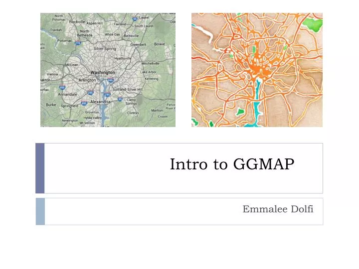
Intro to GGMAP Emmalee Dolfi
Ethical Implications of Spatial Analysis • Spatially displaying data can change how it’s interpreted • Locational privacy and ethics • Volunteered Geographic Information System (VGIS) • Location-based services (LBS) • Data is often collected without the subject knowing it • Radio Frequency Identification (RFID) • Crime Mapping
What is GGMAP? • Spatial visualization with Google Maps, OpenStreetMaps, StamenMaps and CloudMadeMaps • Combine with GGPLOT2 to spatially display data • Use ggmap() to create basemap layer, use “+” to add ggplot2 layer with data HoustonMap <- qmap("houston", zoom = 13, color = "bw") HoustonMap+ geom_point(data=violent_crimes,aes(x = lon, y = lat, colour = offense ) )
Geocoding Your Data • Data must be spatially referenced in order to display it using ggmap
The Process of Geocoding • Assigning a location (latitude, longitude) to an address • Compares elements in the given address the reference data set and finds the best match
Getting a Base Map • Get_map() combines get_googlemap(), get_openstreetmap(), get_stamenmap(), get_cloudmademap() • Arguments: • Center, zoom, maptype, color, source
Displaying Point Data • Geom_point() • Must specify data • Argument: aes() • x = longitude • y = latitude • color = variable to display • If you have factored levels: • Can scale the points based on these factors
Hexagonal Bins • Displays a spatial histogram • Calculates density per bin from point data • Stat_binhex() • Specify data • Need lat and long in aes() • Bins controls the number of bins across the x-axis, which control the size of the bins • Alpha controls transparency
Kernel Density • Calculate magnitude per unit area from point data • Creates equal area cells (like a raster) and gives each cell a value based on the number of point in a “search radius”
References • Michael Mann, Department of Geography, GWU • http://cran.r-project.org/web/packages/ggplot2/ggplot2.pdf • http://cran.r-project.org/web/packages/ggmap/ggmap.pdf • (Movebank.org) Fuller, M.R., Seegar, W.S., and Schueck, L.S. 1998. Routes and Travel Rates of Migrating Peregrine Falcons Falcoperegrinus and Swainson's Hawks Buteoswainsoni in the Western Hemisphere. Journal of Avian Biology 29:433-440. • http://webhelp.esri.com/arcgisdesktop/9.3/index.cfm?TopicName=An_overview_of_geocoding • http://www.cdc.gov/dhdsp/maps/gisx/training/module3/files/2_spatial_analyst_module.PDF