Download
1 / 13
700 likes | 3.03k Views
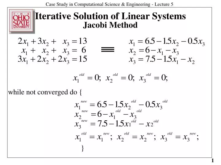
Iterative Solution of Linear Systems Jacobi Method. while not converged do {. }. Gauss Seidel Method. while not converged do {. }. Iterative method can be expressed as: x new =c + Mx old , where M is an iteration matrix. Jacobi : Ax = b, where A = L+D+U, i.e.,

E N D
Iterative Solution of Linear SystemsJacobi Method while not converged do { }
Gauss Seidel Method while not converged do { }
Iterative method can be expressed as: xnew=c + Mxold, where M is an iteration matrix. Jacobi: Ax = b, where A = L+D+U, i.e., (L+D+U)x = b => Dx = b - (L+U)x => x = D-1(b-(L+U)x) = D-1b - D-1 (L+U)x xn+1= D-1(b-(L+U)xn) = c + Mxn Gauss Seidel: (L+D+U)x = b => (L+D)x = b - Ux => xn+1 = (L+D)-1(b-Uxn) = (L+D)-1b - (L+D)-1 Uxn Stationary Iterative Methods
A non-stationary iterative method that is very effective for symmetric positive definite matrices. The method was derived in the context of quadratic function optimization: f(x) = xTAx - 2bx has a minimum when Ax = b Algorithm starts with initial guess and proceeds along a set of orthogonal “search” directions in successive steps. Guaranteed to reach solution (in exact arithmetic) in at most n steps for an nxn system, but in practice gets close enough to solution in far fewer iterations. Conjugate Gradient Method
Steps in CG algorithm in solving system Ax=y: so = r0 =y - Ax0 ak = rkTrk/skTAsk xk+1 = xk +aksk rk+1 = rk -akAsk bk+1 = rk+1Trk+1/rkTrk sk+1 = rk+1 +bk+1sk s is the search direction, r is the residual vector, x is the solution vector; a and b are scalars a represents the extent of move along the search direction New search direction is the new residual plus fraction b of the old search direction. Conjugate Gradient Algorithm
The convergence rate of an iterative method depends on the spectral properties of the matrix, i.e. the range of eigenvalues of the matrix. Convergence is not always guaranteed - for some systems the solution may diverge. Often, it is possible to improve the rate of convergence (or facilitate convergence in a diverging system) by solving an equivalent system with better spectral properties Instead of solving Ax=b, solve MAx = Mb,where M is chosen to be close to A-1. The closer MA is to the identity matrix, the faster the convergence. The product MA is not explicitly computed, but its effect incorporated via an additional matrix-vector multiplication or a triangular solve. Pre-conditioning
Each iteration of an iterative linear system solver requires a sparse matrix-vector multiplication Ax. A processor needs xi iff any of its rows has a nonzero in column i. Communication Requirements P0 P1 P2 P3
The associated graph of a sparse matrix is very useful in determining the communication requirements for parallel sparse matrix-vector multiply. Communication Requirements P0 P0 P1 P2 P1 P3 Comm required: 8 values P2 P0 P1 P2 P3 P3 Alternate mapping: 5 values
Communication for parallel sparse matrix-vector multiplication can be minimized by solving a graph partitioning problem. Minimizing communication
The communication needed for a parallel direct sparse solver is very different from that for an iterative solver. If rows are mapped to processors, comm. is reqd. between procs owning rows j and k (k>j) iff Akj is nonzero. The associated graph of thematrix is not very useful in producing a load-balanced partitioning since it does not capture the temporal dependences in the elimination process. A different graph structure called the elimination tree is useful in determining a load-balanced low-communication mapping. Communication for Direct Solvers
The e-tree is a tree data structure that succintly captures the essential temporal dependences between rows during the elimination process. The parent of node j in the tree is the row# of first non-zero below diagonal in row j (using the “filled-in” matrix). If row j updates row k, k must be an ancestor in the e-tree. Row k can only be updated by a node that is in its subtree. Elimination Tree
Recursive mapping strategy. Sub-trees that are entirely mapped to a processor need no communication between those rows. Subtrees that are mapped amongst a subset of procs only need communication among that group, e.g. rows 36 only needs comm. from P1 Using the E-Tree for Mapping
Direct solvers: Robust: not sensitive to spectral properties of matrix User can effectively apply solver without much understanding of algorithm or properties of matrix Best for 1D problems; very effective for many 2D problems Significant increase in fill-in for 3D problems More difficult to parallelize than iterative solvers; poorer scalability Iterative solvers: No fill-in problem; no explosion of operation count for 3D problems; excellent scalability for large sparse problems But convergence depends on eigenvalues of matrix Preconditioners are very important; good ones usually domain-specific The effectiveness of iterative solvers may require good understanding of mathematical properties of equations in order to derive good preconditioners Iterative vs. Direct Solvers