Download
1 / 84
900 likes | 1.06k Views
What have we leaned so far?. Camera structure Eye structure. Project 1: High Dynamic Range Imaging. What have we learned so far?. Image Filtering Image Warping Camera Projection Model. Project 2: Panoramic Image Stitching. What have we learned so far?. Projective Geometry

E N D
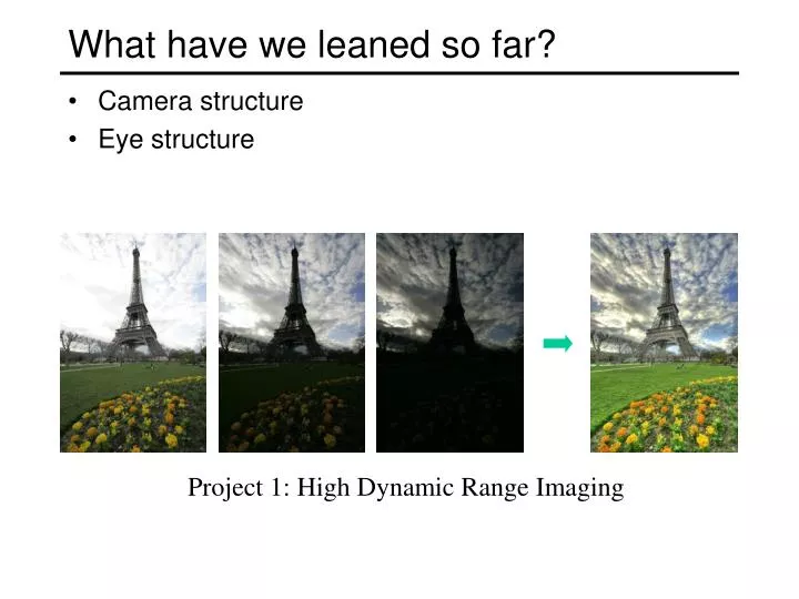
What have we leaned so far? • Camera structure • Eye structure Project 1: High Dynamic Range Imaging
What have we learned so far? • Image Filtering • Image Warping • Camera Projection Model Project 2: Panoramic Image Stitching
What have we learned so far? • Projective Geometry • Single View Modeling • Shading Model Project 3: Photometric Stereo
Today • 3D modeling from two images – Stereo
Public Library, Stereoscopic Looking Room, Chicago, by Phillips, 1923
Inventor: Sir Charles Wheatstone, 1802 - 1875 http://en.wikipedia.org/wiki/Sir_Charles_Wheatstone
Inventor: Sir Charles Wheatstone, 1802 - 1875 http://en.wikipedia.org/wiki/Wheatstone_bridge
Stereograms online • UCR stereographs • http://www.cmp.ucr.edu/site/exhibitions/stereo/ • The Art of Stereo Photography • http://www.photostuff.co.uk/stereo.htm • History of Stereo Photography • http://www.rpi.edu/~ruiz/stereo_history/text/historystereog.html • Double Exposure • http://home.centurytel.net/s3dcor/index.html • Stereo Photography • http://www.shortcourses.com/book01/chapter09.htm • 3D Photography links • http://www.studyweb.com/links/5243.html • National Stereoscopic Association • http://204.248.144.203/3dLibrary/welcome.html • Books on Stereo Photography • http://userwww.sfsu.edu/~hl/3d.biblio.html • A free pair of red-blue stereo glasses can be ordered from Rainbow Symphony Inc • http://www.rainbowsymphony.com/freestuff.html
FUJIFILM, September 23, 2008 Fuji 3D printing
Stereo scene point image plane optical center
Stereo • Basic Principle: Triangulation • Gives reconstruction as intersection of two rays • Requires • calibration • point correspondence
epipolar line epipolar line epipolar plane Stereo correspondence • Determine Pixel Correspondence • Pairs of points that correspond to same scene point • Epipolar Constraint • Reduces correspondence problem to 1D search along conjugateepipolar lines • Java demo: http://www.ai.sri.com/~luong/research/Meta3DViewer/EpipolarGeo.html
Epipolar Line Example courtesy of Marc Pollefeys
Stereo image rectification • reproject image planes onto a common • plane parallel to the line between optical centers • pixel motion is horizontal after this transformation • two homographies (3x3 transform), one for each input image reprojection • C. Loop and Z. Zhang. Computing Rectifying Homographies for Stereo Vision. IEEE Conf. Computer Vision and Pattern Recognition, 1999.
Epipolar Line Example courtesy of Marc Pollefeys
Epipolar Line Example courtesy of Marc Pollefeys
Stereo matching algorithms • Match Pixels in Conjugate Epipolar Lines • Assume brightness constancy • This is a tough problem • Numerous approaches • A good survey and evaluation: http://www.middlebury.edu/stereo/
For each epipolar line For each pixel in the left image Improvement: match windows Basic stereo algorithm • compare with every pixel on same epipolar line in right image • pick pixel with minimum match cost
Basic stereo algorithm • For each pixel • For each disparity • For each pixel in window • Compute difference • Find disparity with minimum SSD
Reverse order of loops • For each disparity • For each pixel • For each pixel in window • Compute difference • Find disparity with minimum SSD at each pixel
Incremental computation • Given SSD of a window, at some disparity Image 1 Image 2
Incremental computation • Want: SSD at next location Image 1 Image 2
Incremental computation • Subtract contributions from leftmost column, add contributions from rightmost column - + - + Image 1 - + - + - + - + - + Image 2 - + - + - +
Selecting window size • Small window: more detail, but more noise • Large window: more robustness, less detail • Example:
Selecting window size 3 pixel window 20 pixel window Why?
Non-square windows • Compromise: have a large window, but higher weight near the center • Example: Gaussian • Example: Shifted windows (computation cost?)
Problems with window matching • No guarantee that the matching is one-to-one • Hard to balance window size and smoothness
A global approach • Finding correspondence between a pair of epipolar lines for all pixels simultaneously
A global approach left right left right left right Define an evaluation score for each configuration, choose the best matching configuration
A global approach • How to define the evaluation score? • How about the sum of corresponding pixel difference?
Ordering constraint • Order of matching features usually the samein both images • But not always: occlusion
Dynamic programming • Treat pixel correspondence as graph problem Right image pixels 1 2 3 4 1 2 Left imagepixels 3 4
1 1 2 2 3 3 4 4 Dynamic programming • Find min-cost path through graph Right image pixels 1 2 3 4 1 2 Left imagepixels 3 4
Energy minimization • Another global approach to improve quality of correspondences • Assumption: disparities vary (mostly) smoothly • Minimize energy function: Edata+lEsmoothness • Edata: how well does disparity match data • Esmoothness: how well does disparity matchthat of neighbors –regularization
Stereo as energy minimization • Matching Cost Formulated as Energy • “data” term penalizing bad matches • “neighborhood term” encouraging spatial smoothness
Energy minimization • Many local minimum • Why? • Gradient descent doesn’t work well • In practice, disparities only piecewise smooth • Design smoothness function that doesn’t penalize large jumps too much • Example: V(a,b)=min(|a-b|, K) • Non-convex
Energy minimization • Hard to find global minima of non-smooth functions • Many local minima • Provably NP-hard • Practical algorithms look for approximate minima (e.g., simulated annealing)
edge weight d3 d2 d1 edge weight Energy minimization via graph cuts Labels (disparities)
d3 d2 d1 Energy minimization via graph cuts • Graph Cost • Matching cost between images • Neighborhood matching term • Goal: figure out which labels are connected to which pixels
d3 d2 d1 Energy minimization via graph cuts • Graph Cut • Delete enough edges so that • each pixel is connected to exactly one label node • Cost of a cut: sum of deleted edge weights • Finding min cost cut equivalent to finding global minimum of energy function
Computing a multiway cut • With 2 labels: classical min-cut problem • Solvable by standard flow algorithms • polynomial time in theory, nearly linear in practice • More than 2 terminals: NP-hard [Dahlhaus et al., STOC ‘92] • Efficient approximation algorithms exist • Yuri Boykov, Olga Veksler and Ramin Zabih, Fast Approximate Energy Minimization via Graph Cuts, International Conference on Computer Vision, September 1999. • Within a factor of 2 of optimal • Computes local minimum in a strong sense • even very large moves will not improve the energy
Red-blue swap move Green expansion move Move examples Starting point
B A AB subgraph (run min-cut on this graph) The swap move algorithm 1. Start with an arbitrary labeling 2. Cycle through every label pair (A,B) in some order 2.1 Find the lowest E labeling within a single AB-swap 2.2 Go there if it’s lower E than the current labeling 3. If E did not decrease in the cycle, we’re done Otherwise, go to step 2 B A Original graph
The expansion move algorithm 1. Start with an arbitrary labeling 2. Cycle through every label A in some order 2.1 Find the lowest E labeling within a single A-expansion 2.2 Go there if it’s lower E than the current labeling 3. If E did not decrease in the cycle, we’re done Otherwise, go to step 2 Multi-way cut A sequence of binary optimization problems
Stereo results • Data from University of Tsukuba scene ground truth http://cat.middlebury.edu/stereo/
Results with window correlation normalized correlation (best window size) ground truth
Results with graph cuts graph cuts (Potts model E, expansion move algorithm) ground truth