Download
1 / 18
290 likes | 1.42k Views
Ch 2 Applications of Quantum Mechanics. Atomic Wave Functions Solving a 3D problem: positively charged nucleus and one negative electron Use methods similar to Particle in a Box to find E and Y For a 1D problem, we generated one quantum number = n

E N D
Ch 2 Applications of Quantum Mechanics • Atomic Wave Functions • Solving a 3D problem: positively charged nucleus and one negative electron • Use methods similar to Particle in a Box to find E and Y • For a 1D problem, we generated one quantum number = n • For a 3D problem, we will generate 3 quantum numbers= n, l, ml • Later, we will add the 4th quantum number to describe e spin (ms) • Quantum Numbers • n = principle quantum number = responsible for Energy of electron • l = orbital angular momentum = responsible for shape of orbital • ml = magnetic angular momentum = responsible for orbital position in space • ms = spin angular momentum = describes orientation of e- magnetic moment • When no magnetic field is present, all ml values have the same energy and both ms values have the same energy • Together, n, l, and ml define one atomic orbital
Conversions: x = r sinq cosf y = r sinq sinf z = r cosq • Spherical Coordinates • Cartesian Coordinates: x, y, z define a point • Spherical Coordinates: r, q, f define a point • r = distance from nucleus for the electron • q = angle from the z-axis (from 0 to p) • f = angle from the x-axis (from 0 to 2p) Spherical Volumes: 3 sides = rdq, r sinq df, and dr V = product = r2 sinq dq df dr Volume of shell between r and r + dr
In Spherical Coordinates, Y is the product of the angular factors • Radial factor describes e- density at different distances from nucleus • Angular factor describes shape of orbital and orientation in space • Y(r,q,f) = R(r)Q(q)F(f) = R(r)Y(qf) [Y combines angular factors] • The Radial Function • R(r) is determined by n, l • Bohr Radius = ao =52.9 pm = r at Y2 maximum probability for a H 1s orbital • Used as a unit of distance for r in quantum mechanics (r = 2ao, etc…) • Radial Probability Function = 4pr2R2 • Describes the probability of finding e- at a given distance over all angles • Plots of R(r) and 4pr2R2 use r scale with ao units • Electron Density falls off rapidly as r increases • For 1s, probability = 0 by the time r = 5ao • For 3d, max prob is at r = 9ao ; prob = 0 at r = 20ao • All orbitals have prob = 0 at the nucleus 4pr2R2 = 0 at r = 0 • Maxima: combination of rapid increase of 4pr2 with r and the rapid decrease of R2 with r • Shape and distance of e- from nucleus determine reactivity (valence)
The Angular Functions • q(q) and F(f) show how the probability changes at the same distance, but different angles = shape/orientation of the atomic orbitals • Angular factors are determined by l and ml • Table 2-2 • Center = shape due to q portion only • Far right = shape due to q and f = 3d orbital shape • Shaded lobes = where Y is negative • Y2 = probability is same for +/-, but useful for bonding
Nodal Surfaces = surfaces where Y2 = 0 (Y changes sign) • Appear naturally from Y mathematical forms • 2s orbital: Y changes sign at r = 2ao giving a nodal sphere • Y2 = prob = 0 for finding the electron here • Y(r,q,f) = R(r)Y(q,f) and Y2 = 0 • Either R(r) = 0 or Y(q,f) = 0 • Determines Nodal Surfaces by finding these conditions • Radial Nodes = Spherical Nodes R(r) = 0 • Gives Layered appearance of orbitals • R(r) changes sign • 1s, 2p, 3d have no radial nodes • Number of radial nodes increases with n • Number of radial nodes = n – l -1
Angular Nodes: Y = 0 = planar or conical • Easiest to see in Cartesian Coordinates (x, y, z) • Can find where Y changes from +/- • Total number of nodes = n - 1 • How can e- have probability on both sides of a nodal plane? • Wave properties • Like a node on a violin string; string still exists even when it has nodes • Example 1 • pz • pz because z appears in the Y expression • Y = 0 for angular node: z = 0 = xy plane is a node • Y = + where z > 0, Y is – where < 0 • 2pz has no spherical nodes
Example 2 • dx2-y2 • Y = 0 when x = y and x = -y • Nodal planes contain z-axis and make 45o angle with x and y axes • Y = + when x2 > y2 and Y = - when x2 < y2 • No spherical nodes • Exercises 2-1 and 2-2 • Linear Combinations • i appears in p and d wave functions • Fortunately, any linear combination of solutions to the Schrodinger Equation is also a solution to the Schrodinger Equation • Simplify p by taking sum and difference of ml = +1 and ml = -1 • Normalize by constants • Now these are real functions (YY* = Y2)
The Aufbau Principle = the Build-Up Principle • Multi-electron atoms have limitations • Any combination of Q#’s works for a 1-electron atom • Electrons will have to interact in multi-electron systems • Rules • Electrons are placed in orbitals to give the lowest energy • Lowest values of n and l filled first • Values of ml and ms don’t effect energy • Pauli Exclusion Principle = every e- has a unique set of quantum numbers • At least on Q# must be different: 2 e- in same orbital have ms = +/- ½ • Not derived from Schrödinger Equation; Experimental Observation • Hund’s Rule = always maximum spin if you have degenerate orbitals • 2 e- in same orbital higher energy than 1 e- each in degenerate orbitals • Electrostatic repulsion explains this (Coulombic Repulsion E = Pc) • Multiplicity = # of unpaired e- + 1 (n + 1)
Exchange Energy = Pe = quantum mechanical result depending on the possible number of exchanges of 2 e- with same E/spin • 2p2 example __ __ __ __ __ __ __ __ __ __ __ __ • P = total pairing E = Pc + Pe Pc = + and approximately constant Pe = - and approximately constant Favors the unpaired configuration vii. Another example p4 and Exercise 2-3 __ __ __ vs. __ __ __ 1Pc – 3Pe 2Pc – 2Pe Lowest E 1 2 2 1 + 1 Pc, 0 Pe 0 Pc, 0Pe 0 Pc, -1Pe Increasing Energy
D) Shielding • Predicting exact order of e- filling is difficult • Shielding Provides an approach to figuring it out • Each e- acts as a shield for e- farther out • This reduces the attraction to the nucleus, increasing E • Figure 2-10 is the accepted energy ordering • n is most important • l does change order for multi-electron systems • As Z increases, the attraction for e- increases and the Energy of the orbitals decreases irregularly • Table 2-6 gives actual e- configurations • Slater’s Rule: Z* = effective nuclear attraction = Z – S • Grouping: 2s,2p/3s,3p/3d/4s,4p/4d/4f/5s5p • e- in higher groups don’t shield lower groups • For ns/np valence e- • e- in same group contributes 0.35 (1s = 0.3) • e- in n-1 group contributes 0.85 • e- in n-2 group contributes 1.00
For nd/nf valence electrons • e- in same group contributes 0.35 • e- in groups to the left contribute 1.00 • S = sum of all contributions • Examples • Oxygen: (1s2)(2s22p4) Z* = Z – S = 8 – 2(0.85) – 5(0.35) = 4.55 Last e- held 4.55/8.00 = 57% of force expected for 8+ nucleus • Nickel: (1s2)(2s22p6)(3s23p6)(3d8)(4s2) Z* = 28 – 10(1.00) – 16(0.85) – 1(0.35) = 4.05 for 4s electron Ni2+ loses 4s2 electrons, not 3d electrons first (d8 metal) c) Exercises 2-4, 2-5 • Why does it work? (Figure 2-6) • 3s,3p 100% shield 3d because their probability is higher than 3d near nucleus = shielding • 2s,2p only shield 3s,3p 85% because 3s/3p have significant regions of high probability near the nucleus
Why are Cr [Ar]4s13d5 and Cu [Ar]4s13d10 • Traditional Explanation: filled and half-filled subshells are particularly stable • Electron Interaction Model • 2 parallel E levels having only one kind of spin • Separated by Pc amount of Energy • E levels slant downward as Z increases (more attraction) • 3d orbitals slant faster than 4s, which has more complete shielding • Fill from bottom up with only e- of one spin type Ti __ __ __ __ __ 3d __ 4s 4s23d2 __ 4s Fe __ __ __ __ __ 3d __ __ __ __ __ 3d __ 4s 4s23d6 __ 4s Cr __ 4s __ __ __ __ __ 3d 4s13d5 __ 4s Cu __ 4s __ __ __ __ __ 3d __ 4s __ __ __ __ __ 3d 4s13d10
Formation of cations: lowers d energy more than s energy, so transition metals always lose s electrons first III. Periodic Properties • Ionization Energy • An+(g) ----> A(n+1)+(g) + e- DU = Ionization Energy • Trends • Increase in DU across period as Z increases so does the attraction to e- • Breaks in trend • B p-orbital 2s22p1 easier to remove • O 2s22p4 paired e- easier to remove __ __ __ • Similar pattern in other periods
Transition Metals have only small differences • Increased shielding • Increased distance from nucleus • Large decreases at start of new period because new s-orbital much higher E • Noble gases decrease as Z increases because e- are farther from nucleus
Electron Affinity • A-(g) ----> A(g) + e- DU = EA • Endothermic except for noble gases and Alkaline Earths • More precisely, this is the Zeroth Ionization Energy • Similar trends to Ionization Energy • Much smaller Energies involved; easier to lose e- from negative charged ion • Ionic Radii • Gradual decrease across a period as Z increases (greater attraction for electrons) 2) General increase down a Group as the size of the valence shell increases 3) Nonpolar Covalent Radii for neutral atoms are found in Table2-7 4) Ionic Radii from crystal data are found in Table 2-8 • Cations are smaller than neutral atoms • Anions are larger than neutral atoms • Radius decreases as + charge increases