Download
1 / 67
670 likes | 679 Views
This course covers various data structures and algorithms including hash tables, heaps, balanced search trees, union-find structures, graphs, B-trees, kD-trees, and more. Learn how to efficiently store and manipulate sets and dictionaries, with applications in compilers, routers, web servers, and more.

E N D
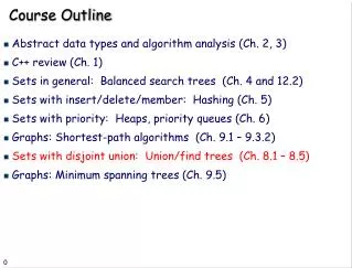
Course Outline • Introduction and Algorithm Analysis (Ch. 2) • Hash Tables: dictionary data structure (Ch. 5) • Heaps: priority queue data structures (Ch. 6) • Balanced Search Trees: general search structures (Ch. 4.1-4.5) • Union-Find data structure (Ch. 8.1–8.5) • Graphs: Representations and basic algorithms • Topological Sort (Ch. 9.1-9.2) • Minimum spanning trees (Ch. 9.5) • Shortest-path algorithms (Ch. 9.3.2) • B-Trees: External-Memory data structures (Ch. 4.7) • kD-Trees: Multi-Dimensional data structures (Ch. 12.6) • Misc.: Streaming data, randomization
Data Structures for Sets • Many applications deal with sets. • Compilers have symbol tables (set of vars, classes) • IP routers have IP addresses, packet forwarding rules • Web servers have set of clients, etc. • Dictionary is a set of words. • A set is a collection of members • No repetition of members • Members themselves can be sets • Examples • {x | x is a positive integer and x < 100} • {x | x is a CA driver with > 10 years of driving experience and 0 accidents in the last 3 years} • All webpages containing the word Algorithms
Abstract Data Types • Set + Operations define an ADT. • A set + insert, delete, find • A set + ordering • Multiple sets + union, insert, delete • Multiple sets + merge • Etc. • Depending on type of members and choice of operations, different implementations can have different asymptotic complexity.
Dictionary ADTs • Data structure with just 3 basic operations: • find (i): find item with key (identifier) i • insert (i): insert i into the dictionary • remove (i): delete i • Just like words in a Dictionary • Where do we use them: • Symbol tables for compiler • Customer records (access by name) • Games (positions, configurations) • Spell checkers • P2P systems (access songs by name), etc.
Naïve Method 1: Linked List • Keep a linked list of the keys • insert (i): add to the head of list. Easy and fast O(1) • find (i): worst-case, search the whole list (linear) • remove (i): also linear in worst-case
Naïve Method 2: Direct Mapping Perm # • An array (bit vector) for all possible keys • Map key i to location i • insert (i): set A[i] = 1 • find (i): return A[i] • remove (i): set A[i] = 0 Student Records Graduates
Naïve Method 2: Direct Mapping • Maintain an array (bit vector) for all possible keys • insert (i): set A[i] = 1 • find (i): return A[i] • remove (i): set A[i] = 0 • All operations easy and fast O(1) • What’s the drawback? • Too much memory/space, and wasteful! • The space of all possible IP addresses, variable names in a compiler is enormous!
Shortcomings of Naïve Implementations • Linked list space-efficient, but search-inefficient. • Insert is O(1) but find and delete are O(n). • A sorted search structure (array) also no good. The search becomes fast, but insert/delete take O(n). • Bit Vector search-efficient but space-inefficient. • Balanced search trees (Chap. 4) work but take O(log n) time per operation, and complicated.
Towards an Efficient Data Structure: Hash Table • Formal Setup • Assume keys are integers {0, 1, …, |U|} • Non-numeric keys (strings, webpages) converted to numbers: Sum of ASCII values, first three characters • The keys come from a known but very large set, called universe U (e.g. IP addresses, program states) • The set of keys to be managed is S is a subset of U. • The size of S is much smaller than U, namely, |S| << |U| • We use n for |S|.
Hash Table • Key idea is that instead of direct mapping, Hash Tables use a Hash Function h to map each input key to a unique location in table of size M • h : U -> {0, 1, …, M-1} • hash function determines the hash table size. • Desiderata: • M should be small, O(n) • h should be easy to compute • Typical example: h(i) = i mod M
Hashing : the basic idea Student Records Perm # (mod 9) Graduates
Hash Tables: Intuition • Hash function lets us find an item in O(1) time. • Each item is uniquely identified by a key • Just check the location h(key) to find the item • Suppose we expect to have at most 100 keys in S • 91, 2048, 329, 17, 689345, …. • We create a table of size 100 and use the hash function h(key) = key mod 100 • It is both fast and uses the ideal size table. • What can go wrong?
Hashing: • But what if all keys end with 00? • All keys will map to the same location • This is called a Collision in Hashing • This motivates the 3rd important property of hashing • A good hash function should evenly spread the keys to foil any special structure of input • Hashing with mod 100 works fine if keys random • Most data (e.g. program variables) are not random
Hashing: • A good hash function should evenly spread the keys to foil any special structure of input • Key idea behind hashing is to “simulate” the randomness through the hash function • A good choice is h(x) = x mod p, for prime p • h(x) = (ax + b) mod p called pseudo-random hash functions
Hashing: The Basic Setup • Choose a pseudo-random hash function h • this automatically determines the hash table size. • An item with key k is put at location h(k). • To find an item with key k, check location h(k). • What to do if more than one keys hash to the same value. This is called collision. • We will discuss two methods to handle collision: • Separate chaining • Open addressing
Maintain a list of all elements that hash to the same value Search using the hash function to determine which list to traverse Insert/deletion–once the “bucket” is found through Hash, insert and delete are list operations Separate chaining 0 1 2 3 4 5 6 7 8 9 10 23 1 56 24 36 14 16 17 7 29 31 20 42 find(k,e)HashVal = Hash(k,Hsize);if (TheList[HashVal].Search(k,e))then return true;else return false; class HashTable { …… private: unsigned int Hsize; List<E,K> *TheList; ……
Insertion: insert 53 0 1 2 3 4 5 6 7 8 9 10 0 1 2 3 4 5 6 7 8 9 10 23 1 56 23 1 56 24 24 36 14 36 14 16 16 17 17 7 29 7 29 53 20 42 31 20 42 31 53 = 4 x 11 + 9 53 mod 11 = 9
Analysis of Hashing with Chaining • Worst case • All keys hash into the same bucket • a single linked list. • insert, delete, find take O(n) time. • A worst-case Theorem later • Average case • Keys are uniformly distributed into buckets • Load Factor L = InputSize/HashTableSize • In a failed search, avg cost is L • In a successful search, avg cost is 1 + L/2
If collision happens, alternative cells are tried until an empty cell is found. Different probing strategies Linear Quadratic Double Hashing Open addressing 0 1 2 3 4 5 6 7 8 9 10 42 1 24 14 16 28 7 31 9
Linear Probing (insert 12) 0 1 2 3 4 5 6 7 8 9 10 42 1 24 14 16 28 7 0 1 2 3 4 5 6 7 8 9 10 42 1 31 24 9 14 12 16 28 7 31 9 12 = 1 x 11 + 1 12 mod 11 = 1
Search with linear probing (Search 15) 0 1 2 3 4 5 6 7 8 9 10 42 1 24 14 12 16 28 7 31 9 15 = 1 x 11 + 4 15 mod 11 = 4 NOT FOUND !
Search with linear probing // find the slot where searched item should be in int HashTable<E,K>::hSearch(const K& k) const { int HashVal = k % D; int j = HashVal; do {// don’t search past the first empty slot (insert should put it there) if (empty[j] || ht[j] == k) return j; j = (j + 1) % D; } while (j != HashVal); return j; // no empty slot and no match either, give up } bool HashTable<E,K>::find(const K& k, E& e) const { int b = hSearch(k); if (empty[b] || ht[b] != k) return false; e = ht[b]; return true; }
Deletion in Hashing with Linear Probing • Since empty buckets are used to terminate search, standard deletion does not work. • One simple idea is to not delete, but mark. • Insert: put item in first empty or marked bucket. • Search: Continue past marked buckets. • Delete: just mark the bucket as deleted.
Deletion with linear probing: LAZY (Delete 9) 0 1 2 3 4 5 6 7 8 9 10 0 1 2 3 4 5 6 7 8 9 10 42 42 1 1 24 24 14 14 12 12 16 16 28 28 7 7 31 31 D 9 9 = 0 x 11 + 9 9 mod 11 = 9 FOUND !
Eager Deletion: fill holes • Remove and find replacement: • Fill in the hole for later searches remove(j) { i = j; empty[i] = true; i = (i + 1) % D; // candidate for swapping while ((not empty[i]) and i!=j) { r = Hash(ht[i]); // where should it go without collision? // can we still find it based on the rehashing strategy? if not ((j<r<=i) or (i<j<r) or (r<=i<j)) then break; // yes find it from rehashing, swap i = (i + 1) % D; // no, cannot find it from rehashing } if (i!=j and not empty[i]) then { ht[j] = ht[i]; remove(i); } }
Eager Deletion Analysis (cont.) • If not full • After deletion, there will be at least two holes • Elements that are affected by the new hole are • Initial hashed location is cyclically before the new hole • Location after linear probing is in between the new hole and the next hole in the search order • Elements are movable to fill the hole Initial hashed location Location after linear probing Initial hashed location Next hole in the search order New hole Next hole in the search order
Eager Deletion Analysis (cont.) • The important thing is to make sure that if a replacement (i) is swapped into deleted (j), we can still find that element. How can we not find it? • If the original hashed position (r) is circularly in between deleted and the replacement i r j r i Will not find i past the empty green slot! j r i i r j Will find i j i i r r
Hashing with Linear Probing • Avg. cost for successful searches ½ (1 + 1/(1 – L)) • Failed search avg. cost more ½ (1 + 1/(1 – L)2)
Quadratic Probing • Solves the clustering problem in Linear Probing • Check H(x) • If collision occurs check H(x) + 1 • If collision occurs check H(x) + 4 • If collision occurs check H(x) + 9 • If collision occurs check H(x) + 16 • ... • H(x) + i2
Quadratic Probing (insert 12) 0 1 2 3 4 5 6 7 8 9 10 42 1 24 14 16 28 7 0 1 2 3 4 5 6 7 8 9 10 42 1 31 24 9 14 12 16 28 7 31 9 12 = 1 x 11 + 1 12 mod 11 = 1
Double Hashing • When collision occurs use a second hash function • Hash2 (x) = R – (x mod R) • R: greatest prime number smaller than table-size • Inserting 12 H2(x) = 7 – (x mod 7) = 7 – (12 mod 7) = 2 • Check H(x) • If collision occurs check H(x) + 2 • If collision occurs check H(x) + 4 • If collision occurs check H(x) + 6 • If collision occurs check H(x) + 8 • H(x) + i * H2(x)
Double Hashing (insert 12) 0 1 2 3 4 5 6 7 8 9 10 42 1 24 14 16 28 7 0 1 2 3 4 5 6 7 8 9 10 42 1 31 24 9 14 12 16 28 7 31 9 12 = 1 x 11 + 1 12 mod 11 = 1 7 –12 mod 7 = 2
Rehashing • If table gets too full, operations will take too long. • Build another table, twice as big (and prime). • Next prime number after 11 x 2 is 23 • Insert every element again to this table • Rehash after a percentage of the table becomes full (70% for example)
Collision Functions • Hi(x)= (H(x)+i) mod B • Linear pobing • Hi(x)= (H(x)+c*i) mod B (c > 1) • Linear probing with step-size = c • Hi(x)= (H(x)+i2) mod B • Quadratic probing • Hi(x)= (H(x)+ i * H2(x)) mod B
Analysis of Open Hashing • Effort of one Insert? • Intuitively – that depends on how full the hash is • Effort of an average Insert? • Effort to fill the Bucket to a certain capacity? • Intuitively – accumulated efforts in inserts • Effort to search an item (both successful and unsuccessful)? • Effort to delete an item (both successful and unsuccessful)? • Same effort for successful search and delete? • Same effort for unsuccessful search and delete?
Issues: • What do we lose? • Operations that require ordering are inefficient • FindMax: O(n) O(log n) Balanced binary tree • FindMin: O(n) O(log n) Balanced binary tree • PrintSorted: O(n log n) O(n) Balanced binary tree • What do we gain? • Insert: O(1) O(log n) Balanced binary tree • Delete: O(1) O(log n) Balanced binary tree • Find: O(1) O(log n) Balanced binary tree • How to handle Collision? • Separate chaining • Open addressing
Theory of Hashing • First the bad news. • Theorem: For any hash function h: U -> {0, 1, …, M}, there exists a set S of n keys that all map to the same location, assuming |U| > nM. • So, in the worst-case no hash function can avoid linear search complexity! • Proof. • Take any hash function h you wish to consider • Map all the keys of U using h to the table of size M • By the pigeon-hole principle, at least one table entry will have n keys. • Choose those n keys as input set S. • Now h will maps the entire set S to a single location, for worst-case example of hashing.
Theory of Hashing • The negative result says that given a fixed hash function h, one can always construct a set S that is bad for h. • However, what we desire is something different: • We are not choosing S; it is our (given) input. • Can we find a good h for this particular S? • Theory shows that a random choice of h works.
Theory of Hashing: Birthday Paradox • To appreciate the subtlety of hashing, first consider a puzzle: the birthday paradox. • Suppose birth days are chance events: • date of birth is purely random • any day of the year just as likely as another
Theory of Hashing: Birthday Paradox • What are the chances that in a group of 30 people, at least two have the same birthday? • How many people will be needed to have at least 50% chance of same birthday? • It’s called a paradox because the answer appears to be counter-intuitive. • There are 365 different birthdays, so for 50% chance, you expect at least 182 people.
Birthday Paradox: the math • Suppose 2 people in the room. • What is the prob. that they have the same birthday? • Answer is 1/365. • All birthdays are equally likely, so B’s birthday falls on A’s birthday 1 in 365 times. • Now suppose there are k people in the room. • It’s more convenient to calculate the prob. X that no two have the same birthday. • Our answer will be the (1 – X)
Birthday Paradox • Define Pi = prob. that first i all have distinct birthdays • For convenience, define p = 1/365 • P1 = 1. • P2 = (1 – p) • P3 = (1 – p) * (1 – 2p) • Pk = (1 – p) * (1 – 2p) * …. * (1 – (k-1)p) • You can now verify that for k=23, Pk <= 0.4999 • That is, with just 23 people in the room, there is more than 50% chance that two have the same birthday
Birthday Paradox: derivation • Use 1 – x <= e-x, for all x • Therefore, 1 – j*p <= e-jp • Also, ex + ey = ex+y • Therefore, Pk <= e(-p -2p -3p … -(k-1)p) • Pk <= e-k(k-1)p/2 • For k = 23, we have k(k-1)/2*365 = 0.69 • e-0.69 <= 0.4999 • Connection to Hashing: • Suppose n = 23, and hash table has size M = 365. • 50% chance that 2 keys will land in the same bucket.
Theory of Hashing: Universal Hash Functions • A set of hash functions H is called universal if for any hash function h chosen randomly from it • Prob[h(x) = h(y)] <= 1/M, for any x, y in U • Theorem. Suppose H is universal, S is an n-element subset of U, and h a random hash function from H. • The expected number of collisions is at most (n-1)/M for any x in S.
Theory of Hashing: Universal Hash Functions • Theorem. Suppose H is universal, S is an n-element subset of U, and h a random hash function from H. • The expected number of collisions is at most (n-1)/M for any x in S. • Proof. • Consider any x in S. For any other y, the prob. that h(y) = h(x) is at most 1/M (by universal hashing) • By linearity of expectation, the number of keys mapping to h(x) is at most (n-1)/M. • Corollary. By using a random hash function (from a universal family), we get expected search time O(1 + n/M). • Universal hash functions exists. Modulo prime is an example, but not proved here.