Download
1 / 20
200 likes | 324 Views
Kalman Filter based Track Fit running on Cell. S. Gorbunov 1,2 , U. Kebschull 2 , I. Kisel 2,3 , V. Lindenstruth 2 and W.F.J. Müller 1 1 Gesellschaft für Schwerionenforschung mbH , Darmstadt, Germany 2 Kirchhoff Institute for Physics, University of Heidelberg, Germany

E N D
Kalman Filter basedTrack Fitrunning on Cell S. Gorbunov1,2, U. Kebschull2, I. Kisel2,3, V. Lindenstruth2 and W.F.J. Müller1 1Gesellschaft für Schwerionenforschung mbH, Darmstadt, Germany 2Kirchhoff Institute for Physics, University of Heidelberg, Germany 3Laboratory of Information Technologies, JINR, Dubna, Russia IBM, Böblingen February 13, 2007
Terminology Kalman FilterbasedTrack Fitrunning on Cell Ivan Kisel, KIP, Uni-Heidelberg
The Kalman Filter 1/3 The filter is named after Rudolf E. Kalman. The Kalman filteris a recursive algorithm which estimates the state of a dynamic system from a series of incomplete and noisy measurements. The filter was developed in papers by Swerling (1958), Kalman (1960), and Kalman and Bucy (1961). An example of an application would be to provide accurate continuously-updated information about the position and velocity of an object given only a sequence of observations about its position, each of which includes some error. It is used in a wide range of engineering applications from radar to computer vision. A wide variety of Kalman filters have now been developed, from Kalman's original formulation, now called the simple Kalman filter, to extended filter, the information filter and a variety of square-rootfilters. Ivan Kisel, KIP, Uni-Heidelberg
Example: Radar Applications 2/3 s2x s2y … s2z s2vx … s2vy s2vz C = In a radar application, where one is interested in following a target, information about the location, speed, and acceleration of the target is measured at different moments in time with corruption by noise. State vector error of x Covariance matrix r = { x, y, z, vx, vy, vz } velocity position December 21, 1968. The Apollo 8 spacecraft has just been sent on its way to the Moon. 003:46:31 Collins: Roger. At your convenience, would you please go P00 and Accept? We're going to update to your W-matrix. Ivan Kisel, KIP, Uni-Heidelberg
The Kalman Filter Algorithm 3/3 n n+1 The Kalman filter is a recursive estimator – only the estimated state from the previous time step and the current measurement are needed to compute the estimate for the current state. mean value over n measurements new measurement previous estimation mean value over n+1 measurements correction weight Update or Filter Prediction or Extrapolation • The Kalman filter exploits the dynamics of the target, which govern its time evolution, to remove the effects of the noise and get a good estimate of the location of the target • at the present time (filtering), • at a future time (prediction), or • at a time in the past (interpolation or smoothing). Ivan Kisel, KIP, Uni-Heidelberg
Terminology Kalman Filter basedTrackFitrunning on Cell Ivan Kisel, KIP, Uni-Heidelberg
The Compressed Baryonic Matter Experiment (GSI, Darmstadt) 1/3 CBM is a typical modern high energy physics experiment Track == trajectory • Challenge: • ~ 1000 charged particles/collision • 107 Au+Au collisions/sec • high speed data acquisition and trigger system Ivan Kisel, KIP, Uni-Heidelberg
Data Acquisition System 2/3 RU RU RU RU RU RU RU RU RU RU RU RU RU RU RU RU 50 kB/ev Detector 107 ev/s 100 ev/slice MAPS STS RICH TRD ECAL SFn Dt SFn Dt SFn Dt SFn Dt SFn Dt Event Builder Network N x M Scheduler SFn Dt MAPS STS RICH TRD ECAL SFn available Farm Control System 5 MB/slice Sub-Farm Sub-Farm Sub-Farm Sub-Farm Sub-Farm Sub-Farm Sub-Farm Sub-Farm Sub-Farm Sub-Farm 105sl/s PC Farm Sub-Farm Sub-Farm Sub-Farm Sub-Farm Sub-Farm Sub-Farm Sub-Farm Sub-Farm Sub-Farm Sub-Farm Sub-Farm Sub-Farm Sub-Farm Sub-Farm Sub-Farm ~1000 PCs … Cell, Cell, Cell, Cell … … Cell, Cell, Cell, Cell … … Cell, Cell, Cell, Cell … … Cell, Cell, Cell, Cell … … Cell, Cell, Cell, Cell … … Cell, Cell, Cell, Cell … … Cell, Cell, Cell, Cell … … Cell, Cell, Cell, Cell … … Cell, Cell, Cell, Cell … … Cell, Cell, Cell, Cell … … Cell, Cell, Cell, Cell … … Cell, Cell, Cell, Cell … … Cell, Cell, Cell, Cell … … Cell, Cell, Cell, Cell … … Cell, Cell, Cell, Cell … Ivan Kisel, KIP, Uni-Heidelberg
Stages of Data Reconstruction 3/3 Track finding Ring finding (PID) Combinatorics Time consuming!!! • Conformal Mapping • Hough Transformation • Track Following + Kalman Filter • Cellular Automaton + Kalman Filter Kalman Filter Track fitting Kalman Filter Vertex finding/fitting Ivan Kisel, KIP, Uni-Heidelberg
Terminology Kalman Filter basedTrackFitrunning on Cell Ivan Kisel, KIP, Uni-Heidelberg
Kalman Filter for Track Fit 1/3 detectors measurements e- (r, C) track parameters and errors Ivan Kisel, KIP, Uni-Heidelberg
The Kalman Filter for Track Fit 2/3 large errors arbitrary non-homogeneous magnetic field as large map multiple scattering in material >>> 256 KB of Local Store weight for update small errors not enough accuracy in single precision Ivan Kisel, KIP, Uni-Heidelberg
Modifications of the Fitting Algorithm 3/3 • The initial track parameters are directly estimated from the input data. • The propagation step is performed directly from measurement to measurement without intermediate steps. • Matrix multiplications have been replaced by direct operations on only non-trivial matrix elements. • Most loops have been unrolled in order to provide additional instructions for interleaving. • All branches have been eliminated from the algorithm to avoid branch misprediction penalty. • Calculations have been reordered for better use of the processors pipeline. Ivan Kisel, KIP, Uni-Heidelberg
Terminology Kalman Filter basedTrackFitrunning on Cell Ivan Kisel, KIP, Uni-Heidelberg
Cell Processor: Supercomputer-on-a-Chip 1/5 • Approach: • Run SPEs independently (one collision per SPE) • Vectorization (SIMDization) • Universality (any CPU architecture) Ivan Kisel, KIP, Uni-Heidelberg
Porting the Kalman Filter on Cell 2/5 Use headers to overload +, -, *, / operators --> the source code is unchanged ! Data Types: • Scalar double • Scalar float • Pseudo-vector (array) • Vector (4 float) c = a + b SSE2 Platform: SSE2 • GSI-Linux • Virtual machine: • Red Hat (Fedora Core 4) • Cell Simulator: • PPE • SPE • Cell Blade AltiVec Specialized SIMD Ivan Kisel, KIP, Uni-Heidelberg
SPE Statistics 3/5 Ivan Kisel, KIP, Uni-Heidelberg
Modifications of the Fitting Algorithm 4/5 Intel P4 Cell Ivan Kisel, KIP, Uni-Heidelberg
Kalman Filter on Intel Xeon, AMD Opteron and Cell 5/5 Fit of a single track: lxg1411 1.7 1.9 eh102 1.6 2.1 blade11bc4 Fit of thousands of tracks: Cell SPE is: 1.5 times faster than Intel Xeon and 2 times faster than AMD Opteron Ivan Kisel, KIP, Uni-Heidelberg
Summary and Plans Sub-Farm … Cell, Cell, Cell, Cell … … Cell, Cell, Cell, Cell … … Cell, Cell, Cell, Cell … ? ? Cellular Automaton Kalman Filter Intel, AMD and Cell Sub-Farm Demonstrator On-line Selection (Trigger) 2. Track Finding 1. Distribution of Data 3. Track Fit Development Ivan Kisel, KIP, Uni-Heidelberg