Download
1 / 21
210 likes | 341 Views
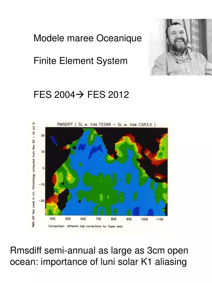
Modele maree Oceanique Finite Element System FES 2004 FES 2012. Rmsdiff semi-annual as large as 3cm open ocean: importance of luni solar K1 aliasing. a: Equilibrium semi-diurnal tides . amplitude. phase. 17cm, M2 8cm, S2. b: Equilibrium diurnal tides . amplitude. phase.

E N D
ModelemareeOceanique Finite Element System FES 2004 FES 2012 Rmsdiffsemi-annual as large as 3cm open ocean: importance of luni solar K1 aliasing
a: Equilibrium semi-diurnal tides amplitude phase 17cm, M2 8cm, S2 b: Equilibrium diurnal tides amplitude phase 10cm, K1 c: M2 and K1 dynamic estimates amplitude amplitude 60cm,M2 24cm,K1 SI- data 1
a: Equilibrium long period tides amplitude phase 3.02 cm, Mf; 1.55 cm, Mm; 1.35 cm, Ssa; 2.07 cm, Sa b: amplitude Mf dynamic estimate 2.8cm c: total tidal transport (kg m2/s) SI- data 2
c: dynamic M2 and K1 tidal amplitudes 60cm,M2 24cm,K1 b: equilibrium long period tides amplitude phase 3 cm, Mf 1.5 cm, Mm c: dynamic Mf tidal amplitude 2.8cm, Mf SI- Data 2
Hemispheric averages of K1 meridional transport N current S S N (cm/s) (m2/s) K1 LuniSolartidal elevation (cm) in Arctic hour hour maxNorthis @12h maxNorth is @16h SI-persp3
Tidal Energy Flux VectorM2K1 Ray et al., 2005 • Semi-diurnal (12h25mn)Diurnal (23h56mn) • Lunar Luni-Solar • Min (1997)/ Max (2006) Lunar Inclinaison • nodal factors: with inclination, K1 increases • 3 times more than M2 decreases • Role K1 increase (18.6yrs) on decadal climate • at high lat where K1 big (Ray, 2007), AND • in tropics because of Yanai increase
a: mean differences: daily TAO (winds) – QSCAT (OVW) Courtesy of Dr. Kelly (OVWST, 2007) b: mean Ocean currents from drifters at 15m NECC SEC SSS SST c: Zonal components d: Meridional components North Trade winds Trade winds QSCAT diff=NECC QSCAT diff=SEC 180ºW…………..longitudes……..90ºW tide diff QSCAT 180ºW………… Longitudes ……..90ºW Equator winds …..……….…. Latitudes …………….. …….. South
Solar climatology of OST (cm) +12 October – April ECCO – (QSCAT) --12 +12 ECCO July-Jan +20 October – April ECCO --12 NORTH average (cm) SOUTH average (cm) --20 O(QSCAT) O(QSCAT) TPJ TPJ month month SI- data4
On average between 25º and 60º latitude: 66% area is ocean in South, 43% area is ocean in South On average between 60º latitudes, North Pac is 22% deeper than South
V transport K1 (m2/s) maxNorth is @16h and is bigger than maxSouth horizontal axis duration = 24h~ K1 tidal cycle (period=23h56mn) =annual cycle for K1 detected by QSCAT or ASCAT Significant phase difference (4hours) between currents and transport North budgets because averaged North Pacific deeper than South. Tidal current values are provided by TPXO7.2 on 1 Nov 2007 from 00h:30 to 23h:30.
a: LOD-moon time series b: LOD_moon wavelet 0.50 days c: LOD_sun wavelet 0.05 days SI- data 5
a: Last and First Quarter around September equinoxes * ~2 weeks apart * ecliptic plane b: New and Full moon during June and December solstices * * ~6 months apart The Earth Moon Mass Center (EMMC) remains in the ecliptic plane. The Earth mass center is 4670 km away from the EMMC.
Energy of the horizontal and vertical acceleration speeds b: meridional c: vertical a: zonal 0.6 days 1.4 days 1.2 days Fig 11
3.5 TW is the tidal power dissipated by the oceans • 3.4 TW is the average total (gas, electricity, etc.) power consumption in US in 2005 • 1.1 TW is the tidal power used by oceans to mix and maintain stratification • 0.7 <-> 1.5 TW is the power induced by OVW stresses in the oceans (90% are dissipated in the upper 100m)
2D Vectors (instant) u , v , w =sqrt(u2+v2) speed Units? Ocean Wind Stress (TX,TY)… Pascal (kg m/s2) Ocean Vectors of Workdone by the (air-sea) Wind Stress on the ocean circulation: (OVWWx,OVWWy) =Sum_surf*time {(TX*u+TY*v) dx.dy.dt} OVWW: the biggest unknown: between 0.4TW and 1.7TW Ocean Tidal Energy (EX,EY)… (kg m2/s) = Sv/m (Ex, Ey) = rg Sum_period{ (u,v)H(h+hs) dt} / period M2:period=12h25mn K1: period=23h56mn S2: period=12h hs=hbody+hload
Tidal astronomic forcingM2K1 semi-diurnal (12h25mn)diurnal (23h56mn semi-diurnal symmetric, diurnal antisymmetric the ocean responses loose symmetry because waters are squeezed to flow between the ocean bottom, its surface and the continents.
QSCAT OVW stress TPJ wave/swell +2.0 3 2 -1.4 1 Tropical Swell pools 100% 72% Indian and Pacific warm pools 32º 24º 13º
mean Sea Level simulated by OGCM forced by QuikSCAT vectors relative to observed MSL model forced by QuikSCAT vectors (CORE2): courtesy of Dr. Large (NCAR), OVWST, 2008 cm The difference between model and observed MSL is too big to be real. It corresponds to a change in Earth’s oblatenesswhich is incompatible with the observed range of LOD variations. New Moon in North around June solstice * * Full Moon In South in June-July 14.7 days apart
What energy vector are detectable by scatterometers for climate? • (U,V) winds in (m/s)… Stress (TX, TY) in (kg/m/s2) = r (u’w’,v’w’) (vertical transfer of turbulent momentum) = r CD Wa (Ua, Va) (CD: drag coefficient) = r CD Wshear (Ushear, Vshear) where (Ushear, Vshear) = (atmosphere – ocean) horizontal flows (Ua-Uo-0.8Uorb) = u*/k ln[….z/z0…] TX (Va-Vo-0.8Vorb) = v*/k ln[….z/z0…] TY where (Uorb, Vorb) =Vector of orbital wave velocities • Energy in (kg*m2/s2): (OVWEx, OVWEy) and (TideOVEx, TideOVEy) (Sum_surf*time {(TX*Uo, TY*Vo) dx.dy.dt } ) (r g Sum_period{(Udx,Vdy) *H*(hT+hTs) ) dt }) 2D- vectors: OVW work rates (per dt, per length) in (kg*m/s3= Watt/m) 1) over which dt do we choose to compute the OVW work rates? 2) over which thickness dz do we choose (u, v) ocean surface? 3) we need the (Uo, Vo) due to p_atmos, tides and fast (TX,TY) as well? 4) we need the work rate via wave/swell too. s0,H1/3 altimeter? Issues so far unresolved due to ocean-air curl/mass discontinuities at interface between 2 thin shells at the surface of the Earth. • Emerging solution: 3D- vectors (OA)Momentum in (kg*m2/s)
a: mean meridional OVW difference: ECMWF - QSCAT b: OVWy stress along 6ºN +0.6 QSCAT62QSCAT65QSCAT66 ERS61 FSU10 NCEP15 +2 dyn/cm2 QSCAT diff tide longitude -2 -0.2 m/s c: zonal averages of meridional winds, QSCAT, differences and tides +1 V tide @ QSCAT (200 kg m2/s) winds VECMWF-VQSCAT (m/s) m/s S Equatpr N latitude -1 60S EQ 60N d: 2000:2004 mean OST: model forced by QSCAT– observations +30 cm -30 SI- data 3