Statistical Learning (From data to distributions)

1. Statistical Learning(From data to distributions)

2. Reminders • HW5 deadline extended to Friday

3. Agenda • Learning a probability distribution from data • Maximum likelihood estimation (MLE) • Maximum a posteriori (MAP) estimation • Expectation Maximization (EM)

4. Motivation • Agent has made observations (data) • Now must make sense of it (hypotheses) • Hypotheses alone may be important (e.g., in basic science) • For inference (e.g., forecasting) • To take sensible actions (decision making) • A basic component of economics, social and hard sciences, engineering, …

5. Candy Example • Candy comes in 2 flavors, cherry and lime, with identical wrappers • Manufacturer makes 5 (indistinguishable) bags • Suppose we draw • What bag are we holding? What flavor will we draw next? H1C: 100%L: 0% H2C: 75%L: 25% H3C: 50%L: 50% H4C: 25%L: 75% H5C: 0%L: 100%

6. Machine Learning vs. Statistics • Machine Learningautomated statistics • This lecture • Bayesian learning, the more “traditional” statistics (R&N 20.1-3) • Learning Bayes Nets

7. Bayesian Learning • Main idea: Consider the probability of each hypothesis, given the data • Data d: • Hypotheses: P(hi|d) h1C: 100%L: 0% h2C: 75%L: 25% h3C: 50%L: 50% h4C: 25%L: 75% h5C: 0%L: 100%

8. Using Bayes’ Rule • P(hi|d) = a P(d|hi) P(hi) is the posterior • (Recall, 1/a = Si P(d|hi) P(hi)) • P(d|hi) is the likelihood • P(hi) is the hypothesis prior h1C: 100%L: 0% h2C: 75%L: 25% h3C: 50%L: 50% h4C: 25%L: 75% h5C: 0%L: 100%

9. P(d|h1)P(h1)=0P(d|h2)P(h2)=9e-8P(d|h3)P(h3)=4e-4P(d|h4)P(h4)=0.011P(d|h5)P(h5)=0.1P(d|h1)P(h1)=0P(d|h2)P(h2)=9e-8P(d|h3)P(h3)=4e-4P(d|h4)P(h4)=0.011P(d|h5)P(h5)=0.1 P(h1|d) =0P(h2|d) =0.00P(h3|d) =0.00P(h4|d) =0.10P(h5|d) =0.90 Sum = 1/a = 0.1114 Computing the Posterior • Assume draws are independent • Let P(h1),…,P(h5) = (0.1,0.2,0.4,0.2,0.1) • d = { 10 x } P(d|h1) = 0 P(d|h2) = 0.2510 P(d|h3) = 0.510 P(d|h4) = 0.7510P(d|h5) = 110

10. Posterior Hypotheses

11. Predicting the Next Draw H • P(X|d) = Si P(X|hi,d)P(hi|d) = Si P(X|hi)P(hi|d) D X Probability that next candy drawn is a lime P(h1|d) =0P(h2|d) =0.00P(h3|d) =0.00P(h4|d) =0.10P(h5|d) =0.90 P(X|h1) =0P(X|h2) =0.25P(X|h3) =0.5P(X|h4) =0.75P(X|h5) =1 P(X|d) = 0.975

12. P(Next Candy is Lime | d)

13. Other properties of Bayesian Estimation • Any learning technique trades off between good fit and hypothesis complexity • Prior can penalize complex hypotheses • Many more complex hypotheses than simple ones • Ockham’s razor

14. Hypothesis Spaces often Intractable • A hypothesis is a joint probability table over state variables • 2n entries => hypothesis space is [0,1]^(2n) • 2^(2n) deterministic hypotheses6 boolean variables => over 1022 hypotheses • Summing over hypotheses is expensive!

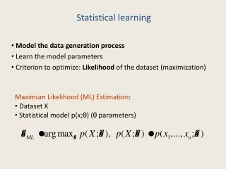
15. Some Common Simplifications • Maximum a posteriori estimation (MAP) • hMAP = argmaxhi P(hi|d) • P(X|d)  P(X|hMAP) • Maximum likelihood estimation (ML) • hML = argmaxhi P(d|hi) • P(X|d)  P(X|hML) • Both approximate the true Bayesian predictions as the # of data grows large

16. Maximum a Posteriori • hMAP = argmaxhi P(hi|d) • P(X|d)  P(X|hMAP) P(X|hMAP) P(X|d) h3 h4 h5 hMAP =

17. Maximum a Posteriori • For large amounts of data,P(incorrect hypothesis|d) => 0 • For small sample sizes, MAP predictions are “overconfident” P(X|hMAP) P(X|d)

18. Maximum Likelihood • hML = argmaxhi P(d|hi) • P(X|d)  P(X|hML) P(X|hML) P(X|d) undefined h5 hML =

19. Maximum Likelihood • hML= hMAP with uniform prior • Relevance of prior diminishes with more data • Preferred by some statisticians • Are priors “cheating”? • What is a prior anyway?

20. Advantages of MAP and MLE over Bayesian estimation • Involves an optimization rather than a large summation • Local search techniques • For some types of distributions, there are closed-form solutions that are easily computed

21. Learning Coin Flips (Bernoulli distribution) • Let the unknown fraction of cherries be q • Suppose draws are independent and identically distributed (i.i.d) • Observe that c out of N draws are cherries

22. Maximum Likelihood • Likelihood of data d={d1,…,dN} given q • P(d|q) = Pj P(dj|q) = qc (1-q)N-c i.i.d assumption Gather c cherries together, then N-c limes

23. Maximum Likelihood • Same as maximizing log likelihood • L(d|q)= log P(d|q) = c log q + (N-c) log(1-q) • maxq L(d|q)=> dL/dq = 0=> 0 = c/q – (N-c)/(1-q)=> q = c/N

24. Maximum Likelihood for BN • For any BN, the ML parameters of any CPT can be derived by the fraction of observed values in the data N=1000 B: 200 E 500 P(E) = 0.5 P(B) = 0.2 Earthquake Burglar A|E,B: 19/20A|B: 188/200A|E: 170/500A| : 1/380 Alarm

25. Maximum Likelihood for Gaussian Models • Observe a continuous variable x1,…,xN • Fit a Gaussian with mean m, std s • Standard procedure: write log likelihoodL = N(C – log s) – Sj (xj-m)2/(2s2) • Set derivatives to zero

26. Maximum Likelihood for Gaussian Models • Observe a continuous variable x1,…,xN • Results:m = 1/N S xj(sample mean)s2 = 1/N S (xj-m)2 (sample variance)

27. Maximum Likelihood for Conditional Linear Gaussians • Y is a child of X • Data (xj,yj) • X is gaussian, Y is a linear Gaussian function of X • Y(x) ~ N(ax+b,s) • ML estimate of a, b is given by least squares regression, s by standard errors X Y

28. Back to Coin Flips • What about Bayesian or MAP learning? • Motivation • I pick a coin out of my pocket • 1 flip turns up heads • Whats the MLE?

29. Back to Coin Flips • Need some prior distribution P(q) • P(q|d) = P(d|q)P(q) = qc (1-q)N-c P(q) Define, for all q, the probability that I believe in q P(q) q 0 1

30. MAP estimate • Could maximize qc (1-q)N-c P(q) using some optimization • Turns out for some families of P(q), the MAP estimate is easy to compute (Conjugate prior) P(q) Beta distributions q 0 1

31. Beta Distribution • Betaa,b(q) = aqa-1 (1-q)b-1 • a, b hyperparameters • a is a normalizationconstant • Mean at a/(a+b)

32. Posterior with Beta Prior • Posterior qc (1-q)N-c P(q)= aqc+a-1 (1-q)N-c+b-1 • MAP estimateq=(c+a)/(N+a+b) • Posterior is also abeta distribution! • See heads, increment a • See tails, increment b • Prior specifies a “virtual count” of a heads, b tails

33. Does this work in general? • Only specific distributions have the right type of prior • Bernoulli, Poisson, geometric, Gaussian, exponential, … • Otherwise, MAP needs a (often expensive) numerical optimization

34. How to deal with missing observations? • Very difficult statistical problem in general • E.g., surveys • Did the person not fill out political affiliation randomly? • Or do independents do this more often than someone with a strong affiliation? • Better if a variable is completely hidden

35. Expectation Maximization for Gaussian Mixture models Clustering: N gaussian distributions Data have labels to which Gaussian they belong to, but label is a hidden variable E step: compute probability a datapoint belongs to each gaussian M step: compute ML estimates of each gaussian, weighted by the probability that each sample belongs to it

36. Learning HMMs Want to find transition and observation probabilities Data: many sequences {O1:t(j) for 1jN} Problem: we don’t observe the X’s! X0 X1 X2 X3 O1 O2 O3

37. Learning HMMs • Assume stationary markov chain, discrete states x1,…,xm • Transition parametersqij = P(Xt+1=xj|Xt=xi) • Observation parametersi = P(O|Xt=xi) X0 X1 X2 X3 O1 O2 O3

38. Learning HMMs • Assume stationary markov chain, discrete states x1,…,xm • Transition parameterspij = P(Xt+1=xj|Xt=xi) • Observation parametersi = P(O|Xt=xi) • Initial statesli = P(X0=xi) x1 q13, q31 x2 x3 3 2 O

39. Expectation Maximization • Initialize parameters randomly • E-step: infer expected probabilities of hidden variables over time, given current parameters • M-step: maximize likelihood of data over parameters x1 q13, q31 x2 x3 P(initial state) P(transition ij) P(emission) q = (1, 2, 3,p11,p12,...,p32p33, 1,2,3) 3 2 O

40. Expectation Maximization q = (1, 2, 3,q11,q12,...,q32q33, 1,2,3) Initialize q(0) E: Compute E[P(Z=z| q(0),O)] Z: all combinations of hidden sequences x1 x2 x3 x2 x2 x1 x1 x1 x2 x2 x1 x3 x2 q13, q31 x2 x3 Result: probability distribution over hidden state at time t 3 2 M: compute q(1) = ML estimate of transition / obs. distributions O

41. Expectation Maximization q = (1, 2, 3,q11,q12,...,q32q33, 1,2,3) Initialize q(0) E: Compute E[P(Z=z| q(0),O)] Z: all combinations of hidden sequences This is the hard part… x1 x2 x3 x2 x2 x1 x1 x1 x2 x2 x1 x3 x2 q13, q31 x2 x3 Result: probability distribution over hidden state at time t 3 2 M: compute q(1) = ML estimate of transition / obs. distributions O

42. E-Step on HMMs • Computing expectations can be done by: • Sampling • Using the forward/backward algorithm on the unrolled HMM (R&N pp. 546) • The latter gives the classic Baum-Welch algorithm • Note that EM can still get stuck in local optima or even saddle points

43. Next Time • Machine learning