Download
1 / 32
320 likes | 500 Views
MSc Module MTMW14 : Numerical modelling of atmospheres and oceans. Modelling the Real World 2.1 Physical parameterisations 2.2 Ocean modelling. Course content. Week 1: The Basics 1.1 Introduction 1.2 Brief history of numerical weather forecasting and climate modelling

E N D
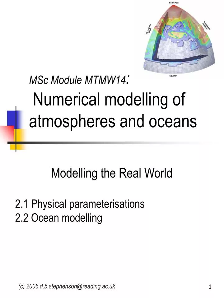
MSc Module MTMW14:Numerical modelling of atmospheres and oceans Modelling the Real World 2.1 Physical parameterisations 2.2 Ocean modelling (c) 2006 d.b.stephenson@reading.ac.uk
Course content Week 1: The Basics 1.1 Introduction 1.2 Brief history of numerical weather forecasting and climate modelling 1.3 Dynamical equations for the unforced fluid Week 2: Modelling the real world 2.1 Physical parameterisations: horizontal mixing and convection 2.2 Ocean modelling Week 3: Staggered schemes 3.1 Staggered time discretisation and the semi-implicit method 3.2 Staggered space discretisations Week 4: More advanced spatial schemes 4.1 Lagrangian and semi-lagrangian schemes 4.2 Series expansion methods: finite element and spectral methods Week 5: Synthesis 5.1 Revision 5.2 Test
2.1 Physical parameterisations The atmosphere and oceans are FORCED DISSIPATIVE fluid dynamical systems: • Q is the fluid dynamics term (dynamical core) • F is forcing and dissipation due to physical • processes such as: • radiation • clouds • convection • horizontal mixing/transport • vertical mixing/transport • soil moisture and land surface processes …
“Earth System” Science, NASA 1986 From Earth System Science – Overview, NASA, 1986
In the Hollow of a Wave off the Coast at Kanagawa", Hokusai 2.1 Unresolved process: horizontal mixing
2.1 Small-scale mixing • Two approaches: • Direct Numerical Simulation (DNS) • try to resolve all spatial scales • using a very high resolution model. • Large-Eddy Simulation (LES) • model the effects of sub-grid scale • eddies as functions of the large-scale • flow (closure parameterisation).
2.1 Horizontal mixing in vorticity eqn Or more correctly model fluxes due to unresolved scales as f(.) + random noise rather than just f(.). (STOCHASTIC PHYSICS)
2.1 Some mixing parameterisations • Diffusion Assume that vorticity flux due to eddies acts to reduce the large-scale vorticity gradient: Note: Mixing isn’t always down-gradient. For example, vorticity fluxes due to mid-latitude storms act to strengthen the westerly jets!
2.1 Some mixing parameterisations • Hyper-diffusion Diffusion is found to damp synoptic features too much. More scale-selective damping can be obtained using: Note: Widely used in spectral models.
2.1 Some mixing parameterisations • Strain-dependent viscosity (Smagorinsky 1963) Put more diffusion in regions that have more large-scale strain: Note: Diffuses more strongly in high strain zones (e.g. between cyclones) but is computationally expensive to implement.
2.1 Spectral blocking and instability In 2-d turbulence and the atmosphere and oceans, enstrophy cascades to ever smaller scales: This cascade can’t continue for ever in numerical models and so in the absence of any mixing parameterisations, energy builds up on the smallest scales. This is known as spectral blocking and can lead to non-linear instability: Phillips, N. A., 1959: An example of nonlinear computational instability. In: B. Bolin (Editor), The Atmosphere and the Sea in Motion. Rockefeller Inst. Press in association with Oxford Univ.Press, New York, 501-504.
2.1 Convection schemes Why parameterise cumulus convection? Precipitation is caused by rising of air due to: • Local convective instability • Large-scale ascent (slantwise convection) • Orographic influences
2.1 Convection schemes Convection occurs on small spatial scales (less than 10km) not explicitly resolvable by weather and climate models. It is important for • producing precipitation and releasing latent heat (diabatic heating of atmosphere). • producing clouds that affect radiation (e.g. cumulonimbus Cb, cumulus Cu, and stratocumulus Sc) • vertical mixing of heat and moisture (and horizontal momentum) Further reading: J. Kiehl’s Chapter 10 in Climate System Modelling (Editor: K. Trenberth) Emanuel, K.A. 1994: Atmospheric convection, Oxford University Press.
2.1 Moist Convective Adjustment Main idea: When model profile (black curve) exceeds moist adiabatic lapse rate at any grid point AND air is fully saturated THEN vertically rearrange temperature and humidity in column so as to lie on a moist adiabat (dashed curve) while conserving moist static energy. All excess moisture is assumed to rain out. Manabe, S., J.Smagorinsky, and R.F.Strickler, 1965: Simulated climatology of a general circulation model with a hydrologic cycle. Mon. Wea. Rev., 93, 769-798.
2.1 MCA assumptions MCA assumes that the intensity of convection is strong enough to eliminate the vertical gradient of potential temperature instantaneously, while conserving total moist static energy. It also assumes that the relative humidity in the layer is maintained at 100%, owing to the vertical mixing of moisture, condensation, and evaporation from water droplets. Good points: simple, quick, works Bad points: instantaneous, ad hoc. Critique: Arakawa, A. and W.H. Schubert, 1974: Interaction of cumulus cloud ensemble with the large scale environment, Part I. J. Atmos. Sci., 31, 674-701. Tiedtke, M., 1989: A comprehensive mass flux scheme for cumulus parameterization in large-scale models. Mon. Wea. Rev., 117, 1799-1800.
2.1 Soft convective adjustment Main idea: Parameterise convection by relaxation terms in the dry static energy and humidity equations. E.g: Betts, A.K. and M.J. Miller, 1986: A new convective adjustment scheme. Part I: Observational & theoretical basis. QJRMS, 112, 677-691. Good points: relaxes gradually to profile, gives more realistic states than MCA Bad points: more tunable parameters (less parsimonious), fixed reference profile
2.1 Mass flux schemes Main idea: Use the cloud properties such as mass flux M determine the relaxation constants. Kuo, H.L., 1974: Further studies of the parameterization of the influence of cumulus convection on large scale flow. J. Atmos. Sci., 31, 1232-1240. Good points: bit more physical Bad points: convection isn’t driven by mass flux but by local instability!
2.1 Summary of main points • Modelling physical processes is an important aspect of weather prediction and climate simulation. Not as simple as modelling the fluid dynamics parts. • Physical schemes take roughly the same amount as computer time as the fluid dynamics schemes. • Forcing (e.g. radiation) and dissipative processes (e.g. mixing) need to be correctly modelled. • Unresolved processes that feedback onto the large-scale flow need to be parameterised in terms of the the large-scale flow.
2.2 Ocean modelling surface currents • Why do we model oceans? • Comparison of oceans and atmosphere • Brief history of ocean modelling Introduction to Physical Oceanography http://gyre.ucsd.edu/sio210/
2.2 Why do we model oceans? • To understand them better! • To understand climate variability better: atmosphere ocean cryosphere • To make environmental predictions (fish) • To hide submarines etc.
2.2 Mid-latitude parameters (450N) • Top 2.5m of ocean have same heat content as 10km of troposphere (factor 4 from C and 1000 from density) • Very different scale heights – most ocean dynamics is in top 1000m and near ocean boundaries • Similar stratification (deep ocean slightly more stable) • Very different Rossby radii oceanic eddies much smaller than atmospheric synoptic systems • Oceans are slow but can transport large volumes: 1 Sverdrup = 1 million cubic metres per second
2.2 Other important differences • Oceans have lateral boundaries so global methods such as spherical harmonics can’t be used • Oceans are heated from above not below (so less convection at low latitudes) • Oceans are rather opaque to electromagnetic radiation • Oceans don’t have clouds but do depend on sea-ice • Sea water isn’t an ideal gas – it’s density is a complicated function of temperature, salinity and pressure. Mixing of two equal density water masses can change the density due to non-linear dependence of density on temperature (cabelling).
2.2 The vorticity equation Exercise: Derive prognostic equations for relative vorticity and divergence using the shallow water equations and compare the resulting vorticity equation to the barotropic vorticity equation. Solution:
2.2 The thermohaline circulation A simple conveyor belt view … But things are a bit more complicated …
2.2 Meridional circulation Time-mean meridional transport streamfunction simulated by a coarse resolution ocean GCM. Contour interval is 4 Sverdrup. From J. McWilliams, in “Ocean modelling and parameterization” by Chassignet and Verron.
2.2 Poleward heat transport Ocean meridional circulation contributes substantially to northward heat transport: From Trenberth (2001) www.cgd.ucar.edu/asr01/Significant.html 1 Petawatt = 1015 Watts
2.2 Brief history of key events • Sverdrup, H.U., 1947: Wind-driven currents in a baroclinic ocean; with application to the equatorial currents of the eastern Pacific. Proc. Nat. Acad. Sci. Wash, 33, 318-326. • Stommel, H.M., 1948. The westward intensification of wind-driven ocean currents. Trans. Amer. Geophys. Union, 29, 202-206. • Bryan, K. 1963: A numerical investigation of a nonlinear model of a wind-driven ocean, J. Atmos. Sci., 20, 594-606. • Bryan, K., and M. D. Cox, 1968: A nonlinear model of an ocean driven by wind and differential heating. Part 1, J. Atmos. Sci., 25, 945-978. - primitive equations for u,v,T,S. rigid lid. Summary of current ocean models: http://www.clivar.org/organization/wgomd/ocean_model.htm More complete historical review: Advances in ocean modeling for climate change research William R Holland, Anatonietta Capodonti, Marika M. Holland http://www.agu.org/journals/rg/rg9504S/95RG00293/index.html
2.2 Summary of main points • Oceans are similar to the atmosphere: differentially rotating stratified fluids • Oceans are different in several ways: • Heated from above • Much denser • Larger heat capacity • Smaller scale height • Oceans are a key component of the climate system (e.g. heat transport) • Ocean modelling has advanced rapidly in the past 50 years • Some key challenges: • Spin-up (> 400 years for Atlantic ocean!) • Resolving synoptic eddies • Parameterising mixing processes • Interaction with sea-ice and atmosphere