Download
1 / 150
1.62k likes | 2.1k Views
Atomic Structure and Periodic Trends. Atomic Structure and Periodic Trends. Lectures: week1: W9 am; week2: W9 am (ICL) & 11 am (DP), F 9 am (DP); week 3: 9 am (ICL) Books: Inorganic Chemistry by Shriver and Atkins Physical Chemistry by P.W.Atkins , J. De Paula

E N D
Atomic Structure and Periodic Trends • Lectures: week1: W9 am; week2: W9 am (ICL) & 11 am (DP), F 9 am (DP); week 3: 9 am (ICL) • Books: • Inorganic Chemistry by Shriver and Atkins • Physical Chemistry by P.W.Atkins , J. De Paula • Essential Trends in Inorganic Chemistry D Mingos • Introduction to Quantum Theory and Atomic Structure by P. A. Cox • Other resources: • Web-pages: http://timmel.chem.ox.ac.uk/lectures/ • Ritchie/Titmuss, Quantum Theory of Atoms and Molecules, Hilary Term
Why study atomic electronic structure? • All of chemistry (+biochemistry etc.) ultimately boils down to molecular electronic structure. • Reason: electronic structure governs bonding and thus molecular structure and reactivity • Before it is possible to understand molecular electronic structure we need to introduce a number of concepts which are more easily demonstrated in atoms. atomic structuremolecular structurechemistry
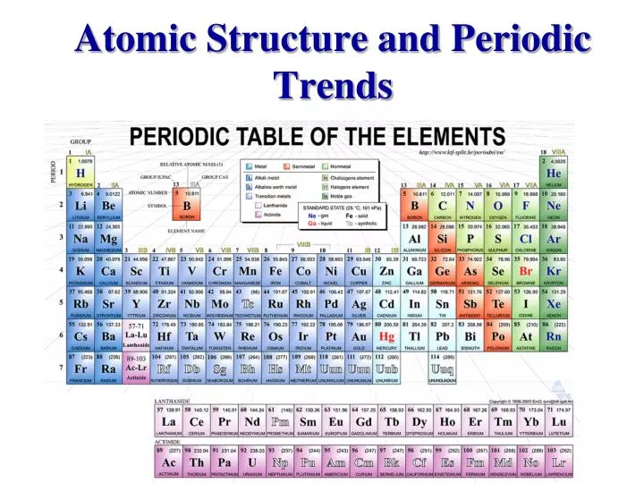
The Periodic Table Mendeleyev, Dmitri Ivanovich (1834-1907) Mendeleyev was the first chemist to understand that all elements are related members of a single ordered system. From his table he predicted the properties of elements then unknown, of which three (gallium, scandium, and germanium) were discovered in his lifetime.
This course...... • will introduce new concepts gradually starting with the “simplest”: H-AtomEnergy levels, Wavefunctions, Born Interpretation, Orbitals Many electron atomsEffects of other electrons, Penetration, Quantum Defect The Aufbau Principle Electronic Configuration of atoms and their ions Trends in the PT Ionisation Energy, Electron Affinity, Size of atoms and ions
The H-Atom 1 H 1.008
v - + r The Hydrogen Atom • The simplest possible system and the basis for all others: Electron orbits the proton under the influence of the Coulomb Force: Revision
- + r H-Atom: consider the energy v ETotal = c.m.
Energy Levels? • Consider 3 approaches: • Classical • Bohr Model (old quantum theory) • Full Quantum: Schrödinger Equation
Classically: • There is no theoretical restriction at all on v or r (there are infinitely many combinations with the same energy). • Hence the energy can take any value - it is . • As a result transitions should be possible everywhere across the electromagnetic spectrum. • So lets see the spectrum...
+ lens lens H2 screen - prism Infra- red Ultra-violet XUV visible The H-atom Emission Spectrum
Principles of Quantum Mechanics Quantization Energy levels
The Rydberg Formula Revision In 1890 Rydberg showed that the frequencies of all transitions could be fit by a single equation:
4 3 2 1 n Bohr Theory (old quantum) • Bohr explained the observed frequencies by restricting the allowed orbits the electron could occupy to particular circular orbits(by quantizing the angular momentum). • His theory gives energy levels:
The problem with Bohr Theory • Bohr theory works extremely well for the H-atom. • However; • it provides no explanation for the quantization of energy -it just happens to fit the observed spectrum But, more seriously: • it just doesn’t work at all for any other atoms
Quantum mechanical Principlesand the Solution of the Schrödinger Equation
Principles of Quantum Mechanics Quantization Quantum mechanics Classical mechanics Energy levels is continuous
Principles of Quantum MechanicsIt’s all about probability In classical mechanics Position of object specified In quantum mechanics Only of object at a particular location
Principles of Quantum MechanicsHow do we describe the electrons in atoms? e- You know: Electrons can be described as (characterised by mass, momentum, position…) p = h/l De Broglie However: Electrons can also be described as (characterised by wavelength, frequency, amplitude) and show properties such as interference, diffraction h = Planck’s constant = 6.626 10-34 Js
The Davisson Germer Experiment Proving the wave properties of electrons (matter!) Intensity variation in diffracted beam shows constructive and destructive interference of wave
Principles of Quantum Mechanics The Wavefunction In quantum mechanics, an electron, just like any other particle, is described by a Important Y(position, time) Contains all information there is to know about the particle
Schrödinger equation: where The Results of Quantum Mechanics More on than in Hilary Term is the wavefunction, V(r) the potential energy and E the total energy
r Spherical Polar Coordinates • Instead of Cartesian (x,y,z) the maths works out easier if we use a different coordinate system: x = r sin cos y = r sin sin z = r cos z y (takes advantage of the spherical symmetry of the system) x
as before with But now where So Schrödinger’s Equation becomes..... More on than in Hilary Term
....which can be solved exactly for the H-atom with the solutions called orbitals, more specifically, atomic orbitals. • We separate the wavefunction into 2 parts: • a radial part R(r) and • an angular part Y(,), such that = • The solution introduces 3 quantum numbers: Important
....which can be solved exactly for the H-atom with the solutions called orbitals, more specifically, atomic orbitals. • We separate the wavefunction into 2 parts: • a radial part R(r) and • an angular part Y(,), such that =R(r)Y(,) • The solution introduces 3 quantum numbers: Important
The quantum numbers; • quantum numbers arise in the solution; • R(r) gives rise to: the principal quantum number, n • Y(,) yields: the orbital angular momentum quantum number, l and the magnetic quantum number, ml i.e., =Rn,l(r)Yl,m(,) Important
The values of n, l, & ml n = 1, 2, 3, 4, ....... l = 0, 1, 2, 3, ......(n-1) ml = -l, -l+1, -l+2,..0,..., l-1, l Important
You are familiar with these..... • nis the integer number associated with an orbital • Different l values have different names arising from early spectroscopy e.g.,l =0 is labelled l =1 is labelled l =2 is labelled l =3 is labelled etc... Important
Looked at another way..... n =1 l=0 ml=01s orbital (1 of) n =2 l=0 ml=0 2s orbital (1 of) l=1 ml=-1, 0, 1 2p orbitals (3 of) n =3 l=0 ml=03s orbital (1 of) l=1 ml=-1, 0, 13p orbitals (3 of) l=2 ml=-2,-1,0,1,23d orbitals (5 of) etc. etc. etc. Hence we begin to see the structure behind the periodic table emerge. Important
Exercise 1; Work out, and name, all the possible orbitals with principal quantum number n=5. How many orbitals have n=5?
The Radial Wavefunctions • The radial wavefunctions for H-atom are the set of Laguerre functions in terms of n, l a0 (=0.05292nm) is the -the most probable orbital radius ofan H-atom 1s electron.
R(r) 1s R(r) 2p 2s Important R(r) 3s 3p 3d
Revisit: The Born Interpretation 2 Y* = Y The square of the wavefunction, at a point is proportional to the of finding the particle at that point. Y* is the complex conjugate of Y. In 1D: If the amplitude of the wavefunction of a particle at some point x isY(x) then the probability of finding the particle between x and x +dx is proportional to 2 (x)Y*(x)dx= (x) dx
R(r)2 R(r) 1s 1s 2p 2p 2s 2s 3p 3s 3p 3d 3d 3s
At long distances from the nucleus, all wavefunctions decay to . Some wavefunctions are zero at the nucleus (namely, all but the l=0 (s) orbitals). For these orbitals, the electron has a zero probability of being found . Some orbitals have nodes, ie, the wave function passes through zero; There are such radial nodes for each orbital.
In 3D: If the amplitude of the wavefunction of a particle at some point (x,y,z) isY(x,y,z) then the probability of finding the particle between x and x+dx, y+dyandz+dz, ie, in a volume dV = dxdydzis given by Y(x,y,z) dV 2 It follows therefore that z 2 Y(x,y,z) dz dy dx is a probability density. y In spherical coordinates 2 Y(r,q,f) x
More important to know probability of finding electron at a given distance from nucleus! …..in a shell of z dz dy y dx Cartesian coordinates not very useful to describe orbitals! x dA=dxdy dA = r2sinqdfdq Surface element dV=dxdydz dV = r2sinqdfdqdr Volume element
For spherically symmetric orbitals: the radial distribution function is defined as 2 P(r)= 4pr2 Y(r) and P(r)dr is the probability of finding the electron in a shell of radius r and thickness dr
Construction of the radial distribution function For spherically symmetrical orbitals P(r)
Radial distribution function P(r) Born interpretation prob = Y2dt Hence plot P(r) = r2R(r)2 P(r)=4pr2Y2 (for spherical symmetry) Pn(r) has nodes Important
So what do we learn? R(r) R(r)2 r r P(r) The 2p orbital is on average closer to the nucleus, but note the 2s orbital’s high probability of being r
3d vs 4s P(r)
The Angular Wavefunction The Ylm(,) angular part of the solution form a set of functions called the n.b. These are generally imaginary functions -we use real linear combinations to picture them.
The Shapes of Wavefunctions (Orbitals) • Shapes arise from combination of radial R(r) and angular parts Ylm(,)of the wavefunction. • Usually represented as boundary surfaces which include of the probability density. The electron does not undergo planetary style circular orbits. • These are the familiar spherical s-orbitals and dumbell-shaped p-orbitals, etc... Important
Electron densities representations The s-orbitals: R2 * R2 R(r) R(r) r - - + + Important + Signs of corresponding wave functions of corresponding wave functions (white areas) * Please note that R and R2 are arbitrarily scaled.
Boundary Model Boundary model of an s orbital within which there is 90% probability of finding the electron
The p-orbitals: boundary surfaces - actually imaginary functions but linear combinations give the familiar dumbells Different shades denote different signs of the wavefunction Important px py pz One Nodal plane