INTRODUCTION

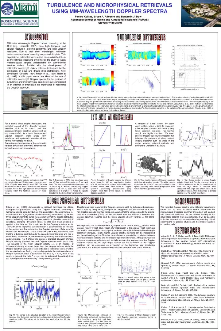
1. TURBULENCE AND MICROPHYSICAL RETRIEVALS USING MM-WAVELENGTH DOPPLER SPECTRA Pavlos Kollias, Bruce A. Albrecht and Benjamin J. Dow Rosenstiel School of Marine and Atmospheric Science (RSMAS), University of Miami INTRODUCTION TURBULENCE RETRIEVALS Millimeter wavelength Doppler radars operating at 94 GHz (e.g. Lhermitte 1987); have high temporal and spatial resolution, extreme sensitivity, and high velocity resolution. Due to their short wavelength, millimeter radars are capable of detecting very small droplets. This capability of millimeter wave radars has established them as the ultimate observing systems for the study of weak meteorological targets undetectable by conventional weather radars. Parallel with the development of millimeter wavelength radars, retrieval techniques for the estimation of cloud and drizzle drop distributions were developed (Gossard 1994; Frisch et al., 1995; Babb et al., 1999). In this paper, some new ideas on the use of millimeter wavelength Doppler spectra for the retrieval of turbulence and microphysical parameters are considered in an attempt to emphasize the importance of recording the Doppler spectrum. In the case of fair-weather cumuli and non-drizzling stratus layers, cloud droplets are the main source of backscattering. The terminal velocity of a cloud droplet is small, (0.3 cm s-1 and 7 cm s-1 for a 10µm and a 50µm droplet, respectively) so that the droplets’ vertical velocity is primarily due to air motion and turbulence. The cloud droplets’ inertia is small so they are good tracers of turbulent air velocity in the same way that smoke particles reveal turbulent eddies in a smoke filled room. The time-height mapping of the mean Doppler velocity reveals the cloud internal circulation structure in terms of updrafts-downdrafts (Kollias and Albrecht, 2000; Kollias et al., 2001) that can use to analyze the internal dynamics and the interaction between the cloud and its environment. Examples of Large-Eddy Observations (LEO, Figs. 1-3), power spectra of vertical velocity time series (Fig. 4) and calculations of fractional area of updrafts and downdrafts (Fig. 5) using direct sampling or the statistics of the vertical velocity (Randall et al., 1992) in a non-drizzling marine stratus are shown in the above figures. I/Q AND MICROSHEAR For a typical cloud droplet distribution, the expected spread of the droplets’ terminal velocities (0.3 to 10 cms-1) and the associated Doppler spectrum variance will be only a few cm2s-2. As a result the observed Doppler spectrum width arises from turbulence and systematic variation of the vertical wind across the beam. Depending on the character of the systematic variation of w across the beam, either wide or bimodal spectra can be produced. A variation of 2 ms-1 across the beam cross section, which is likely to happen in a fair weather cumulus, will create a very large spectrum variance. Fair-weather cumuli are highly turbulent. We often observe Doppler spectrum bimodality that indicates the presence of sharp vertical velocity gradients such as those in the region between adjacent updrafts and downdrafts (Albrecht et al, 2001). Fig. 6: Mean Doppler velocity estimates using FFT calculated using raw I/Q time series in a cirrus cloud. 2,500 I/Q pairs were used for each FFT. The data were collected within (black) and above (red) a cirrus fallstreak. Notice the high-resolution mean Doppler variability within the fallstreak caused by micro-shear. Fig. 7: Examples of FFTs (top) calculated using raw I/Q time series (2,500 pairs – 0.5 sec dwell time). The data correspond to the time period 26-30 sec in Fig. 6. Bottom: The resulting Doppler spectra if all the I/Q data were used for the calculation of a single FFT. Notice the spectra broadening due to the linear variation of w. Fig. 8: Simulation of Doppler spectra for different types (linear (top left) and step-function (bottom left)) of sub-resolution volume cross-radial wind variation. Linear wind fields result in Doppler spectrum broadening. Discontinuous (step function) wind field profile results in bimodal Doppler spectrum. Fig. 9: Time-height mapping of Doppler spectrum width in a fair-weather cumulus. The white contour represents the 1.5 ms-1 contour identified as the updraft boundary. Note the large spectrum width values near the updraft boundary. Fig. 10 Top: Cross section of mean Doppler velocity (blue) and Doppler spectrum width at 1.55 km altitude within the fair weather cumuli. Note the large values of spectrum width associated with large wind shear zones at the updraft boundaries. Bottom: Example of bimodal spectra near the updraft boundaries. MICROPHYSICAL RETRIEVALS CONCLUSIONS Frisch et al., (1995) demonstrate a retrieval technique for drizzle microphysical parameters using the Doppler moments. Assuming a lognormal drizzle size distribution, the parameters (N-concentration, ro-modal radius and x-lognormal distribution width) are retrieved by the first three Doppler moments. While the assumption that the drizzle distribution controls reflectivity and mean Doppler velocity is plausible, especially if conditional sampling (threshold values for dBZ and mean Doppler) is applied to the data set, this is not clear for the Doppler spectrum width. The width of the lognormal size distribution is parameterized as the ratio of the second and first moment of the Doppler spectrum. Data from the Drizzle and Entrainment Cloud Study 99 (DECS’99) experiment show that the turbulence contribution to the second moment is large and has to be removed. Otherwise, x and N will be significantly overestimated and ro underestimated. Fig. 1 shows time series of standard deviation of mean Doppler velocity (dashed line) and Doppler spectrum width (solid line). The variance of the mean Doppler velocity 2w is an indicator of turbulence intensity at scales larger than the sampled volume, while the Doppler spectrum variance 2 is an indicator of turbulence intensity within the sampled volume. During non-drizzling periods the main contributor to Doppler spectrum width is turbulence and thus t = Rw (R1 in our case). In general, the ratio R = t/w can be estimated theoretically from the Kolmogorov turbulence theory. During drizzling periods: 2 = 2t + 2DSD. Therefore we need to correct the Doppler spectrum width for turbulence broadening. This is done by using the w during the drizzling period and the estimate of R from non-drizzling periods. In other words, we assume that the variance due to the drizzle drop size distribution (DSD) can be estimated from the difference between the Doppler spectrum variance and the mean Doppler velocity variance at the same altitude: The recorded Doppler spectra from millimeter wavelength radars can be used to obtain critical information on microphysical processes and their interaction with updraft and downdraft structures. As the retrieval techniques for cloud radar become more sophisticated, it will be possible to further advance our understanding by providing critical observations for process studies and the direct evaluation of cloud models. The lognormal size distribution width x is given at the ratio of the DSD and the mean Doppler velocity (Frisch et al., 1995). Our modification to the original Frisch technique can lead to more realistic microphysical retrievals since the turbulence broadening is essentially removed. Finally, higher Doppler spectra moments can be incorporated into the retrieval algorithm. The data have showed a remarkable correlation between the mean Doppler velocity and the Doppler spectrum skewness. Although turbulence acts as a smearing mechanism and partially removes the asymmetry of the Doppler spectrum caused by the large drops velocity tail, the skewness of the Doppler spectrum can be expressed as a function of the lognormal size distribution parameters and therefore can be used to enhance the robustness of the retrievals. REFERENCES Albrecht, B. A., P. Kollias and B. J. Dow, 2001. Millimeter-wavelength radar observations of updrafts, downdrafts and turbulence in fair weather cumuli, 30th International Conference on Radar Meteorology, Munich, Germany, 19-24 July 2001. Babb, D., J. Verlinde and B.A. Albrecht, 1999. Retrieval of cloud microphysical parameters from 94-GHz radar Doppler power spectra. J. Atmos. Oceanic Tech., 16, 489-503. Gossard E. E., 1994: Measurements of cloud droplet size spectra by Doppler radar. J. Atmos. Oceanic Tech., 11, 712-726 Frisch, A.S., C.W. Fairall and J.B. Snider, 1995. Measurement of stratus cloud and drizzle parameters in ASTEX with a K –band Doppler radar and microwave radiometer. J. Atmos. Sci., 52, 2788-2799. Istok, M.J. and R.J. Doviak, 1986. Analysis of the relation between doppler spectral width and thunderstorm turbulence. J. Atmos. Sci., 42, 607-614. Kollias, P. and B.A. Albrecht, 2000. The turbulent structure in a continental stratocumulus cloud from millimeter-wavelength radar observations. J. Atmos. Sci., 57, 2417-2434. Kollias, P., B.A. Albrecht, R. Lhermitte and A. Savtchenko 2001. Radar Observations of Updrafts, Downdrafts, and Turbulence in Fair Weather Cumuli. J. Atmos. Sci., 58, 1750-1766. Randall, D. A., Q. Shao, and C-H Moeng, 1992: A second order bulk boundary-layer model. J. Atmos. Sci., 49, 1903-1923. Figure 13: Modal radius time series of the drizzle modal radius (m) at gate 3, 260 m over the time interval 13:20 UTC to 14:30 UTC. Fig. 11 Time series of the standard deviation of the mean Doppler velocity (average time 5 minutes) (dashed line) and standard deviation of the Doppler spectrum (solid). The circles at the top of the graph show the drizzling periods. Figure 12: Microphysical retrievals of drizzle modal radius (m), number density (lt-1), logarithmic width (x), and liquid water content (gm-3). The data from the radar at each gate are averaged over the time interval 13:40 UTC to 13:45 UTC. Fig. 14: Time series of Mean Doppler velocity and Doppler spectrum skewness during a drizzling period.