Background – Maxwell Equations

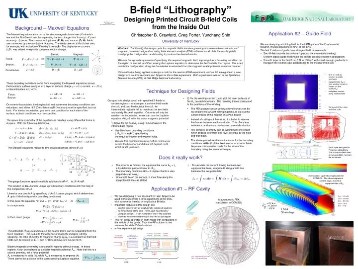
1. Bt=0 on ends so solution is axially symmetric • equipotentials M=cform winding traces for current on face n£(H=rM) • end plates connect along inside/outside • 3-d layout of flux return and inner coils Abstract: Traditionally the design cycle for magnetic fields involves guessing at a reasonable conductor and magnetic material configuration, using finite element analysis (FEA) software to calculate the resulting field, modifying the configuration, and iterating to produce the desired results. We take the opposite approach of specifying the required magnetic field, imposing it as a boundary condition on the region of interest, and then solving the Laplace equation to determine the field outside that region. The exact conductor configuration along the boundaries is extracted from the magnetic scalar potential in a trivial manner. This method is being applied to design a coils for the neutron EDM experiment, and an RF waveguide in a new design of a neutron resonant spin flipper for the n-3He experiment. Both experiments will run at the Spallation Neutron Source (SNS) at Oak Ridge National Laboratory.  +             • 2) Fix the winding current I0 and plot the level surfaces of the Ám on each boundary. The resulting traces correspond to the positions of the winding. • The FEA postprocessor-generate level curves can be fed directly into a CAM milling machine, to cut out the current traces of the magnet on a PCB board. • Instead of cutting out thin wires, it is better to remove thin traces between each conductor. This offers less resistance, and a more continuous current distribution. • Any complex geometry can be wound with one circuit which bridges over from one level potential to the next and then back. • The above procedure does not account for the boundary conditions n£H= K of the fixed interior or exterior fields. Separate coils must be made for this side of the boundary using the same technique.   • Our goal is to design a coil with specified B-fields in certain regions – for example: a uniform field inside the coil, and zero field outside the coil. An intermediate region is left to match up the two fields and satisfy Maxwell equation. Currents will only be used on the boundaries, so we can use the Laplace equation r2Ám=0 with the scalar magnetic potential. • 1) Solve for the field Ám using FEA software in the intermediate region • Use Neumann boundary conditions ( Ám/n = n¢B/¹) specified by the required interior and exterior fields. • We use this condition because n¢B is continuous across the boundary and does not depend on K, which is still unknown.                                                         Top view beam right  J   y -metal shield 10 Gauss solenoid 1010 steel flux return B Im  supermirror bender polarizer (transverse) Ker z Im FnPB cold neutron guide Ker x    • The proof is as follows: the equipotential curve Ám = Inis by definition perpendicular to rÁm. • The boundary condition n£H= K implies that K is also perpendicular to rÁm. • Since both lie on the surface, K must flow along the equipotential lines as stated. • To calculate the current flowing between two equipotential lines, integrate K along a field line between the two potentials: beam left Im Ker Im Ker 3He Beam Monitor transition field (not shown) RF spinrotator 3He target / ion chamber FNPB n-3He B-field “Lithography” Designing Printed Circuit B-field Coils from the Inside Out Background – Maxwell Equations Application #2 – Guide Field Christopher B. Crawford, Greg Porter, Yunchang Shin University of Kentucky The Maxwell equations arise out of the electromagnetic force laws (Coulomb’s law and the Biot-Savart law) by separating the two charges into force (’, J’) and source (, J) terms. The corresponding force (E, B) and source (D, H) fields are connected by the constitutive relations. The fields take on a life of their own, for example, with inclusion of Faraday’s law (tB). The displacement current (tD)was added to explicitly conserve electric charge. • We are designing a holding field for the UCN guide of the Fundamental Neutron Physics Beamline (FnPB) at the SNS • The last 2 metres of guide have stringent field requirements: • Zero B-field outside the coil (can’t perturb the mu-metal shielding) • Uniform dipole guide field inside the coil (to preserve neutron polarization) • Smooth taper in the field from 5 G to 100 mG with small enough gradients to transport the neutron spin adiabatically to the measurement cell Electric Magnetic Force: Source: Constitutive: These boundary conditions come from integrating the Maxwell equations across the boundary surface (along n) of a layer of surface charge , current or discontinuities in ²,¹,or ¾. Technique for Designing Fields Force: Source: On exterior boundaries, the longitudinal and transverse boundary conditions are redundant, and either n£E (Dirichlet) or n¢D (Neuman) must be specified, but not both. For interior boundaries, you have one condition for each side of the surface, so both conditions must be specified. The space-time symmetry of the equations is manifest using differential forms in 4-space. With the following definitions, The Maxwell equations reduce to two exact sequences (since d2=0): Field taper designed to Preserve adiabaticity. The curvature field lines are unavoidable, but can Be minimized. Does it really work? 3-d model of tapered coil calculated in COMSOL. The ribons represent current loops, placed at equipotentials of Ám The gauge functions specify multiple solutions to dA=F, ie. A’=A+dÂ. The solution to dG=J and is unique up to boundary conditions with the help ofthe complement dF=0. Likewise one can fix A by specifying d*A=0 (Lorenz gauge), which determines  up to 2Â=0 (unique with boundary conditions) In this case the equation *d* dA = (2 - d *d*) A = *J or 2A= -J . In components: Application #1 – RF Cavity • We are designing a new resonant RF spin flipper to be used in the upcoming n-3He experiment at the SNS, with transverse instead of longitudinal B-fields. • Important features in this design are: • Can flip transversely or longitudinally polarized neutrons • No fringe fields at the end – 100% spin flip efficiency • Compact design – it can fit inside of the n-3He solenoid • Matches the driver electronics of the NPDG spin flipper • The RF cavity operates in TEM mode with conductors in the middle of the guide. Thus the RF solution is the same as the static B-field solution. • n-3He experimental setup: 0 m – 100 mG 1 m – 189 mG 2 m – 460 mG 3 m – 2.4 G 4 m ~ 10 G Magnetostatic FEA calculation in COMSOL jmax =152 A/m Pmax =11.3W/m2 P~ 100 W 1.16 A 50 windings NPDGamma windings In the Lorenz gauge, n-3He windings The potentials (Á,A) exists because the source terms can be separated from the force equation. This is due to the absence of magnetic charges. Strictly speaking, the ratio of electric to magnetic charge qe/qm is a constant so that field fields can be rotated in (E,H) and (D,B) to remove one source term. Electric/magnetic symmetry is restored in regions without charge. In those regions, A can be replaced by a scalar magnetic potential Ám. Note that this is a source potential, not a force potential. Áe is measured in volts (V), while Ám is measured in amperes (A). There cannot be a source in the corresponding Laplace equation. red - transverse B-field lines blue - end-cap windings