Download
1 / 32
330 likes | 483 Views
Chapter 3: Interactions and Implications. Start with Thermodynamic Identities.

E N D
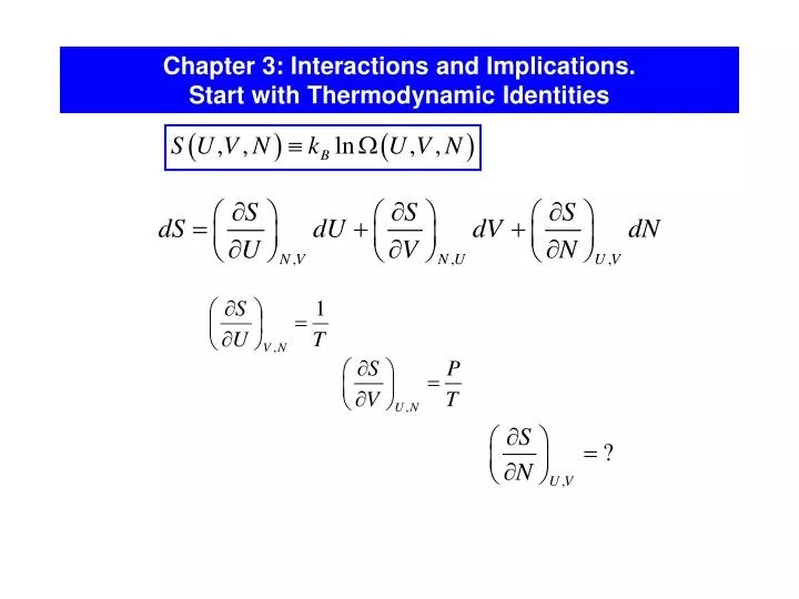
Chapter 3: Interactions and Implications.Start with Thermodynamic Identities
Let’s fix VA and VB (the membrane’s position is fixed),but assume that the membrane becomes permeable for gas molecules (exchange of both U and N between the sub-systems, the molecules in A and B are the same ). Diffusive Equilibrium and Chemical Potential For sub-systems in diffusive equilibrium: UA, VA, NA UB, VB, NB In equilibrium, - the chemical potential Sign “-”: out of equilibrium, the system with the larger S/N will get more particles. In other words, particles will flow from from a high /T to a low /T.
Chemical Potential: examples Einstein solid: consider a small one, with N = 3 and q = 3. let’s add one more oscillator: To keep dS = 0, we need to decrease the energy, by subtracting one energy quantum. Thus, for this system Monatomic ideal gas: At normal T and P, ln(...) > 0, and < 0 (e.g., for He, ~ - 5·10-20 J ~ - 0.3 eV. Sign “-”: usually, by adding particles to the system, we increase its entropy. To keep dS = 0, we need to subtract some energy, thus U is negative.
The Quantum Concentration n=N/V – the concentration of molecules 0 when n increases The chemical potential increases with the density of the gas or with its pressure. Thus, the molecules will flow from regions of high density to regions of lower density or from regions of high pressure to those of low pressure . when n nQ, 0 - the so-called quantum concentration (one particle per cube of side equal to the thermal de Broglie wavelength). When nQ >> n, the gas is in the classical regime. At T=300K, P=105 Pa , n << nQ. When n nQ, the quantum statistics comes into play.
Entropy Change for Different Processes The partial derivatives of S play very important roles because they determine how much the entropy is affected when U, V and N change: The last column provides the connection between statistical physics and thermodynamics.
Thermodynamic Identity for dU(S,V,N) if monotonic as a function of U (“quadratic” degrees of freedom!), may be inverted to give pressure chemical potential compare with shows how much the system’s energy changes when one particle is added to the system at fixed S and V. The chemical potential units – J. - the so-called thermodynamic identity for U This holds for quasi-static processes (T, P, are well-define throughout the system).
Thermodynamic Identities - the so-called thermodynamic identity With these abbreviations: shows how much the system’s energy changes when one particle is added to the system at fixed S and V. The chemical potential units – J. is an intensive variable, independent of the size of the system (like P, T, density). Extensive variables (U, N, S, V ...) have a magnitude proportional to the size of the system. If two identical systems are combined into one, each extensive variable is doubled in value. The thermodynamic identity holds for the quasi-static processes (T, P, are well-define throughout the system) The 1st Law for quasi-static processes (N = const): This identity holds for small changes Sprovided T and P are well defined. The coefficients may be identified as:
The Equation(s) of State for an Ideal Gas Ideal gas: (fN degrees of freedom) The “energy” equation of state (U T): The “pressure” equation of state (P T): - we have finally derived the equation of state of an ideal gas from first principles! In other words, we can calculate the thermodynamic information for an isolated system by counting all the accessible microstates as a function of N, V, and U.
Ideal Gas in a Gravitational Field Pr. 3.37. Consider a monatomic ideal gas at a height z above sea level, so each molecule has potential energy mgz in addition to its kinetic energy. Assuming that the atmosphere is isothermal (not quite right), find and re-derive the barometric equation. note that the U that appears in the Sackur-Tetrode equation represents only the kinetic energy In equilibrium, the chemical potentials between any two heights must be equal:
2 P S =const along the isentropic line 2* 1 Vf Vi V Caution: for non-quasistatic adiabatic processes, S might be non-zero!!! Pr. 3.32.A non-quasistatic compression. A cylinder with air (V = 10-3 m3, T = 300K, P =105 Pa) is compressed (very fast, non-quasistatic) by a piston (A = 0.01 m2, F = 2000N, x = 10-3m). Calculate W, Q, U, and S. An example of a non-quasistatic adiabatic process holds for all processes, energy conservation quasistatic, T and P are well-defined for any intermediate state quasistatic adiabatic isentropic Q = 0 for both non-quasistatic adiabatic The non-quasistatic process results in a higher T and a greater entropy of the final state.
Direct approach: adiabatic quasistatic isentropic adiabatic non-quasistatic
2 To calculate S, we can consider any quasistatic process that would bring the gas into the final state (S is a state function). For example, along the red line that coincides with the adiabata and then shoots straight up. Let’s neglect small variations of T along this path ( U << U, so it won’t be a big mistake to assume T const): P U = Q = 1J 1 Vf Vi V The entropy is created because it is an irreversible, non-quasistatic compression. 2 P For any quasi-static path from 1 to 2, we must have the same S. Let’s take another path – along the isotherm and then straight up: U = Q = 2J isotherm: 1 Vf Vi V “straight up”: Total gain of entropy:
The inverse process, sudden expansion of an ideal gas (2 – 3) also generates entropy (adiabatic but not quasistatic). Neither heat nor work is transferred: W = Q = 0 (we assume the whole process occurs rapidly enough so that no heat flows in through the walls). 2 P Because U is unchanged, T of the ideal gas is unchanged. The final state is identical with the state that results from a reversible isothermal expansion with the gas in thermal equilibrium with a reservoir. The work done on the gas in the reversible expansion from volume Vf to Vi: 3 1 Vf Vi V The work done on the gas is negative, the gas does positive work on the piston in an amount equal to the heat transfer into the system Thus, by going 1 2 3 , we will increase the gas entropy by
Systems with a “Limited” Energy Spectrum The definition of T in statistical mechanics is consistent with our intuitive idea of the temperature (the more energy we deliver to a system, the higher its temperature) for many, but not all systems.
S T S U water ice vapor T U “Unlimited” Energy Spectrum the multiplicity increase monotonically with U : U f N/2 self-gravitating ideal gas (not in thermal equilibrium) Pr. 3.29. Sketch a graph of the entropy of H20 as a function of T at P = const, assuming that CP is almost const at high T. ideal gas in thermal equilibrium S Pr. 1.55 U At T0, the graph goes to 0 with zero slope. At high T, the rate of the S increase slows down (CP const). When solid melts, there is a large S at T = const, another jump – at liquid–gas phase transformation. U T T > 0 T > 0 U C C U
S U E “Limited” Energy Spectrum: two-level systems e.g., a system of non-interacting spin-1/2 particles in external magnetic field. No “quadratic” degrees of freedom (unlike in an ideal gas, where the kinetic energies of molecules are unlimited), the energy spectrum of the particles is confined within a finite interval ofE (just two allowed energy levels). 2NB the multiplicity and entropy decrease for some range of U S U in this regime, the system is described by a negative T T U Systems with T < 0 are “hotter” than the systems at any positive temperature - when such systems interact, the energy flows from a system with T < 0 to the one with T > 0 .
½ Spins in Magnetic Field N - the number of “up” spins N - the number of “down” spins The magnetization: E E2 = + B an arbitrary choice of zero energy 0 The total energy of the system: E1 = - B - the magnetic moment of an individual spin Our plan: to arrive at the equation of state for a two-state paramagnet U=U(N,T,B) using the multiplicity as our starting point. (N,N) S (N,N)= kB ln (N,N) U=U (N,T,B)
From Multiplicity – to S(N)and S(U) The multiplicity of any macrostate with a specified N: Max. S at N = N (N= N/2): S=NkBln2 ln2 0.693
Energy E E From S(U,N) – to T(U,N) The same in terms of N andN : Boltzmann factor!
Energy E2 E1 Energy E2 E2 E1 E1 The Temperature of a Two-State Paramagnet T= + and T= - are (physically) identical – they correspond to the same values of thermodynamic parameters. E2 T E1 E2 E1 N B 0 U - N B Systems with neg. T are “warmer” than the systems with pos. T: in a thermal contact, the energy will flow from the system with neg. T to the systems with pos. T.
E6 E5 E4 E3 E2 B E1 T = 0 The Temperature of a Spin Gas The system of spins in an external magnetic field. The internal energy in this model is entirely potential, in contrast to the ideal gas model, where the energy is entirely kinetic. Boltzmann distribution At fixed T, the number of spins niof energy Eidecreases exponentially as energy increases. B spin 5/2 (six levels) Ei Ei Ei Ei the slope T T = no T - lnni - lnni - lnni - lnni For a two-state system, one can always introduce T - one can always fit an exponential to two points. For a multi-state system with random population, the system is out of equilibrium, and we cannot introduce T.
The Energy of a Two-State Paramagnet (N,N) S (N,N)= kB ln (N,N) U=U (N,T,B) The equation of state of a two-state paramagnet: U U NB B/kBT T 1 - NB - NB U approaches the lower limit (-NB) as T decreases or, alternatively, B increases (the effective “gap” gets bigger).
S NkBln2 S(B/T) for a Two-State Paramagnet U Problem 3.23 Express the entropy of a two-state paramagnet as a function of B/T . - N B 0 N B
S(B/T) for a Two-State Paramagnet (cont.) B/T 0, S = NkB ln2 B/T , S = 0 high-T (low-B) limit S/NkB ln2 0.693 ln2 0.693 low-T (high-B) limit kBT/B = x-1
Low-T limit Which x can be considered large (small)? ln2 0.693
The Heat Capacity of a Paramagnet The low-T behavior: the heat capacity is small because when kBT << 2 B, the thermal fluctuations which flip spins are rare and it is hard for the system to absorb thermal energy (the degrees of freedom are frozen out). This behavior is universal for systems with energy quantization. The high-T behavior:N ~ N and again, it is hard for the system to absorb thermal energy. This behavior is not universal, it occurs if the system’s energy spectrum occupies a finite interval of energies. 2 B kBT 2 B kBT C NkB/2 compare with Einstein solid equipartition theorem (works for quadraticdegrees of freedom only!) E per particle
N B/kBT - N The Magnetization, Curie’s Law The magnetization: M The high-T behavior for all paramagnets (Curie’s Law) N 1 B/kBT
Negative T in a nuclear spin system NMR MRI Fist observation – E. Purcell and R. Pound (1951) An animated gif of MRI images of a human head. -Dwayne Reed Pacific Northwest National Laboratory By doing some tricks, sometimes it is possible to create a metastable non-equilibrium state with the population of the top (excited) level greater than that for the bottom (ground) level - population inversion. Note that one cannot produce a population inversion by just increasing the system’s temperature. The state of population inversion in a two-level system can be characterized with negative temperatures - as more energy is added to the system, and S actually decrease.
Metastable Systems without Temperature (Lasers) For a system with more than two energy levels, for an arbitrary population of the levels we cannot introduce T at all - that's because you can't curve-fit an exponential to three arbitrary values of #, e.g. if occ. # = f (E) is not monotonic (population inversion). The latter case – an optically active medium in lasers. E4 Population inversion between E2 and E1 E3 E2 E1 Sometimes, different temperatures can be introduced for different parts of the spectrum.
Problem • A two-state paramagnet consists of 1x10²² spin-1/2 electrons. The component of the electron’s magnetic moment along B is B = 9.3x10⁻²⁴ J/T. The paramagnet is placed in an external magnetic field B = 1T which points up. • Using Boltzmann distribution, calculate the temperature at which N= N/e. • Calculate the entropy of the paramagnet at this temperature. • What is the maximum entropy possible for the paramagnet? Explain your reasoning. spin 1/2 (two levels) (a) B B - B E2 = + BB kBT E1= - BB
Problem (cont.) If your calculator cannot handle cosh’s and sinh’s: S/NkB 0.09 kBT/ B
Problem (cont.) the maximum entropy corresponds to the limit of T (N=N): S/NkB ln2 (b) For example, at T=300K: E2 kBT E1 ln2 S/NkB T S/NkB ln2 T 0 S/NkB 0 kBT/ B