Download

1 / 39
430 likes | 585 Views
GENERATING STOCHASTIC VARIATES . we discuss techniques for generating random numbers with a specific distribution Random numbers following a specific distribution are called random variates or stochastic variates. The inverse transformation method .

E N D
we discuss techniques for generating random numbers with a specific distribution • Random numbers following a specific distribution are called random variatesor stochastic variates
The inverse transformation method • This method is applicable only to cases where the cumulative density function can be inversed analytically. • CDF? • The proportion of population with value less than x • • The probability of having a value less than x
The inverse transformation method • We wish to generate a stochastıc varieties, from a PDF f(x) • F(x) cdf [0, 1] • FIRST generate random s= F(x) • x=F-1(r)
Example • We want to generate random variates with probability density function • f(x)=2x, 0≤x≤1 • =x2 0≤x≤1 , • Let r be a random number. We have • r=x2,
Sampling from continuous-time probability distributions • We will use invers transform technique to generate variates from a • uniform distribution, • an exponential distribution, and • an Erlang distribution.
Sampling from a uniform distribution • probability density function
Unifrom Cont. • d
Varyansnedir • Olasılık kuramı ve istatistik bilim dallarında varyans • bir rassal değişken, bir olasılık dağılımı veya örneklem için istatistiksel yayılımın, • mümkün bütün değerlerin • beklenen değer veya ortalamadan uzaklıklarının karelerinin ortalaması şeklinde bulunan bir ölçüdür • Ortalama bir dağılımın merkezsel konum noktasını bulmaya çalışırken, varyans değerlerin ne ölçekte veya ne derecede yaygın olduklarını tanımlamayı hedef alır. • Varyansiçin ölçülme birimi orijinal değişkenin biriminin karesidir. Varyansın kare kökü standart sapma olarak adlandırılır; bunun ölçme birimi orijinal değişkenle aynı birimde olur ve bu nedenle daha kolayca yorumlanabilir.
Inverse CDF • sd
Sampling from an exponential distribution • The probability density function of the exponential distribution is defined as follows: • Cumulative Density Function
Exponantial Dist. • expectation and variance are given
INVERSE TRANS. Since 1-F(x) is uniformly distributed in [0,1], we can use the following short-cut procedure
AgnerKrarupErlang • AgnerKrarupErlang (1 January 1878 – 3 February 1929) was a Danish mathematician,statistician and engineer, who invented the fields of traffic engineering and queueing theory. • By the time of his relatively early death at the age of 51, Erlang created the field of telephone networks analysis. His early work in scrutinizing the use of local, exchange and trunk telephone line usage in a small community to understand the theoretical requirements of an efficient network led to the creation of the Erlang formula, which became a foundational element of present day telecommunication network studies.
Sampling from an Erlang distribution • In many occasions an exponential distribution may not represent a real life situation • execution time of a computer program, • manufacture an item • It can be seen, however, as a number of exponentially distributed services which take place successively • If the mean of each of these individual services is the same, then the total service time follows an Erlangdistribution
Erlang • The Erlang distribution is the convolution of k exponential distributions having the same mean 1/a • An Erlang distribution consisting of k exponential distributions is referred to as Ek • The expected value and the variance of a random variable X that follows the Erlang distribution are:
Erlangvariates may be generated by simply reproducing the random process on which the Erlang distribution is based. • This can be accomplished by taking the sum of k exponential variates, x1, x2, ..., xk with identical mean 1/a.
Sampling from discrete-time probability distributions • Geometric Distribution • Binomial Distribution • Poisson Distribution
Geometric Distribution • Consider a sequence of independent trials, where the outcome of each trial is either a failure or a success. • Let p and q be the probability of a success and failure respectively. We have that p+q=1. • The random variable that gives the number of successive failures that occur before a success occurs follows the geometric distribution • PDF Expectation • CDF Variance
Applying Inverse Transform to obtain geometric variates • since p=1-q => • F(n)=1-qn+1 • 1-F(n)=qn+1 • Since 1-F(n) changes [0,1] let r be random number • r=qn+1 (take inverse of CDF)
Alternatively • since (1-F(n))/q=qn, and (1-F(n))/q varies between 0 and 1
Recap Bernoulli trials • In the theory of probability and statistics, a Bernoulli trial (or binomial trial) is a random experiment with exactly two possible outcomes, "success" and "failure", in which the probability of success is the same every time the experiment is conducted. • A random variable corresponding to a binomial is denoted by B(n, p), and is said to have a binomial distribution. The probability of exactly k successes in the experiment B(n, p)is given by: For a fair coin the probability of exactly two tosses out of four total tosses resulting in a heads is given by:
Sampling from a binomial distribution • Consider a sequence of independent trials (Bernoulli trials). • expectation and variance of the binomial distribution are:
Cont. • We can generate variates from a binomial distribution with a given p and n as follows. • We generate n random numbers, after setting a variable k0 equal to zero. For each random number ri, i=1, 2, ..., n, a check is made, and the variable kiis incremented as follows: • The final quantity kn is the binomial variate. This method for generating variates is known as the rejection method.
Sampling from a Poisson distribution • The Poisson distribution models the occurrence of a particular event over a time period. • Let λbe average of number of occurrence during a unit time. Then, the number of occurrence x during a unit period has the following probability density function • P(n)=e-λ(λn/n!) n=0, 1, 2, … • it can be demonstrated that the time elapsing between two successive occurrences of the event is exponentially distributed with mean 1/λ, f(t)=λ e-λt
Poisson Variates • One method for generating Poisson variates involves the generation of exponentially distributed time intervals • t1, t2, t3,... • with an expected value equal to 1/λ. • These intervals are accumulated until they exceed 1, the unit time period. That is,
The Stochastic variates n simply the number of events occurred during a unit time period. Now, since ti = -1/λ log ri , n can be obtained by simply summing up random numbers until the sum for n+1 exceeds the quantity e-λ. That is, n is given by the following expression:
Sampling from an empirical probability distribution • Quite often an empirical probability distribution may not be approximated satisfactorily by one of the well-known theoretical distributions. In such a case, one is obliged to generate variates which follow this particular empirical probability distribution. In this section, we show how one can sample from a discrete or a continuous empirical distribution.
Sampling from a discrete-time probability distribution • Let X be a discrete random variable, • p(X = i) = pi, where pi is calculated from empirical data. • Let p(X≤i) = Pi be the cumulative probability • Let r be a random number , r falls between P2 and P3 • the random variate • x is equal to 3. • if Pi-1<r<Pi then x=i. This method is based on the fact that pi=Pi-Pi-1and that since r is a random number, it will fall in the interval (Pi, Pi-1) pi% of the time.
Example • let us consider the well-known newsboy problem. Let X be the number of newspapers sold by a newsboy per day. From historical data We have, • The cumulative probability distribution is:
Sampling from a continuous-time probability distribution • Let us assume that the empirical observations of a random variable X can be summarized into the histogram • xi is the midpoint of the ith interval, and f(xi) is the length of the ith rectangle. • approximately construct the cumulative probability distribution
The cumulative distribution is assumed to be monotonically increasing within each interval [F(xi-1), F(xi)].
Let r be a random number and let us assume that F(xi-1)<r<F(xi). Then, using linear interpolation, the random variate x can be obtained as follows: • http://en.wikipedia.org/wiki/Linear_interpolation
The rejection method • The rejection technique can be used to generate random variates, if f(x) is bounded and x has a finite range, say a ≤ x ≤ b. The following steps are involved: 1. Normalize the range of f(x) by a scale factor c so that cf(x)≤1,a≤x≤b. (See figure 3.8) 2. Define x as a linear function of r, i.e. x = a + (b-a) r, where r is a random number. 3. Generate pairs of random numbers (r1, r2). 4. Accept the pair and use x = a + (b-a)r1 as a random variate whenever the pair satisfies the relationship r2 ≤ cf(a + (b-a)r1), i.e. the pair (x,r2) falls under the curve in figure 3.8.
Problem • Use the inverse transformation method to generate random variates with probability density function
Problem2 • Apply the inverse transformation method and devise specific formulae that yield the value of variate x given a random number r. (Note that f(x) below needs to be normalized.)
Bibliography • http://www.math.vt.edu/people/qlfang/class_home/Lesson2021.pdf CDF • http://en.wikipedia.org/wiki/Agner_Krarup_Erlang • http://tr.wikipedia.org/wiki/Varyans • http://en.wikipedia.org/wiki/Bernoulli_trial