Download
1 / 30
320 likes | 527 Views
Mixing. Shear Production. Buoyancy Production. z 1. To mix the water column, kinetic energy has to be converted to potential energy. Mixing increases the potential energy of the water column. z 2. z. Mixing vs. Stratification. Potential energy of the water column:.

E N D
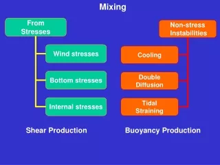
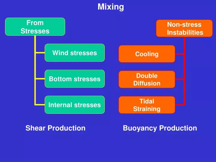
Mixing Shear Production Buoyancy Production
z1 To mix the water column, kinetic energy has to be converted to potential energy. Mixing increases the potential energy of the water column z2 z Mixing vs. Stratification
Potential energy of the water column: Potential energy per unit volume: But The potential energy per unit area of a mixed water column is: Ψ has units ofenergy per unit area
z1 z2 If z no energy is required to mix the water column The energy difference between a mixed and a stratified water column is: with units of [ Joules/m2 ] φ is the energy required to mix the water column completely, i.e., the energy required to bring the profile ρ(z) to ρhat It is called the POTENTIAL ENERGY ANOMALY It is a proxy for stratification The greater the φ the more stratified the water column
We’re really interested in determining whether the water column remains stratified or mixes as a result of the forcings acting on the water column. For that we need to study [ Watts per squared meter ]
De Boer et al (2008, Ocean Modeling, 22, 1) Bx and By are the along-estuary and cross-estuary straining terms Ax and Ay are the advection terms Cx and Cy interaction of density and flow deviations in the vertical C’x and C’y correlation between vertical shear and density variations in the vertical; depth-averaged counterparts of C E is vertical mixing and D is vertical advection Hx and Hy are horizontal dispersion; Fs and Fb are surface and bottom density fluxes
1-D idealized numerical simulation of tidal straining Burchard and Hofmeister (2008, ECSS, 77, 679)
destratified @ end of flood stratified entire period Burchard and Hofmeister (2008, ECSS, 77, 679)
De Boer et al (2008, Ocean Modeling, 22, 1) Bx and By are the along-estuary and cross-estuary straining terms Ax and Ay are the advection terms Cx and Cy interaction of density and flow deviations in the vertical C’x and C’y correlation between vertical shear and density variations in the vertical; depth-averaged counterparts of C E is vertical mixing and D is vertical advection Hx and Hy are horizontal dispersion; Fs and Fb are surface and bottom density fluxes
The power/unit area generated by the wind at a height of 10 m is given by: But the power/unit area generated by the wind stress on the sea surface is: W* is the wind shear velocity at the surface and equals: Mixing Power From Wind
Alternatively, δ is a mixing efficiency coefficient = 0.023 ksis a drag factor that equals 6.4x10⁻⁵ or( Cd u / W ) Mixing Power From Wind (cont.)
But only a fraction of this goes to mixing Mixing Power From Tidal Currents Can also be expressed in terms of bottom stress. The power/unit area produced by tidal flow interacting with the bottom is: ε is a mixing efficiency [ 0.002, 0037 ] Cb is a bottom drag coefficient = 0.0025
Considering advection of mass by ‘u’ only: assuming the along-estuary density gradient is independent of depth, i.e., Tidal Straining We need u(z) from tidal currents to determine the power to stratify/destratify from tidal straining
Taking, (Bowden and Fairbairn, 1952, Proc. Roy. Soc. London, A214:371:392.) 1.15 0.72 Tidal Straining (cont.)
The water column will stratify at ebb as is positive, and vice versa Tidal Straining (cont.)
Taking again: and using Gravitational Circulation will tend to stratify the water column
α is the thermal expansion coefficient of seawater ~ 1.6x10⁻⁴ °C-1 cp is the specific heat of seawater ~ 4x10³ J/(kg °C) Q is the cooling/heating rate (Watts/m2) Heating/Cooling In addition to buoyancy from heating, it may come from precipitation (rain) Δρ is the density contrast between fresh water and sea water Pris the precipitation rate (m/s)
The alternative way of representing the riverine influence on stratification is by assuming that increased R enhances Δρ / Δx. This may be parameterized with Assuming that each stratifying/destratifying mechanism can be superimposed separately: In estuaries, however, the main input of freshwater buoyancy is from river discharge. There is no simple way of dealing with feshwater input as specified by the discharge rate R because R is not distributed uniformly over a prescribed area (as is the case for wind, bottom stress, rain, heat). Caution! Increased R does not necessarily mean increased gradients
α = 1.6x10⁻⁴ °C-1 cp = 4x10³ J/(kg °C) H = 10 m If the contrast between rain water and sea water is 20 kg/m3, then Example: Let’s compare the stratifying tendencies of rain as compared to a low heating rate of 10 W/m2 A precipitation rate of 1.7 mm per day is comparable to a heating rate of 10 W/m2 Where can this happen?
If stratification remains unaltered (or if buoyancy = mixing), For a prescribed Q, the only variables are H and u0 Competition between buoyancy from Heating and mixing from Bottom Stress If Q increases, u0 needs to increase to keep H/u03constant If u0 does not increase then stratification ensues H/u03is then indicative of regions where mixed waters meet stratified
Simpson-Hunter parameter H/u03 ~ 1.6x10⁴/ Q Line where mixed waters are separated from stratified waters. LOG10 (H / U3)
Loder and Greenberg, 1996, Cont. Shelf Res., 6(3), 397-414. M2 ----------------- M2-N2 ------------ M2-N2-S2-------- M2+N2+S2------
Restrictions of the approach? Dominant Stratifying Power from Heating Dominant Destratifying Power from bottom stresses
In order to balance that stratifying power, we need a wind power of: or a current power of: Another example: Assume a system with Δρ / Δx of 10 kg/m3 over 50 km = 2x10⁻⁴, H = 10 m, Az =0.005 m2/s
In order to balance such stratifying power, we need a wind power of: or a current power of: Another example: Assume a system with Δρ / Δx of 1 kg/m3 over 3 km, H = 20 m, Av =0.001 m2/s
Examples of successful applications of this approach: Simpson et al. (1990), Estuaries, 13(2), 125-132. Lund-Hansen et al. (1996), Estuar. Coast. Shelf Sci., 42, 45-54.