Download

1 / 39
470 likes | 1.18k Views
Airborne Weather Radars. Airborne Weather Radars. Outline Research radars on NOAA and NCAR aircraft Scientific “roles” Sampling considerations for wind field analysis Basic Idea Single-Doppler Dual-Doppler Quad-Doppler Editing Doppler radar data Synthesizing Doppler radar data

E N D
Airborne Weather Radars M. D. Eastin
Airborne Weather Radars • Outline • Research radars on NOAA and NCAR aircraft • Scientific “roles” • Sampling considerations for wind field analysis • Basic Idea • Single-Doppler • Dual-Doppler • Quad-Doppler • Editing Doppler radar data • Synthesizing Doppler radar data • Interpolating data to Cartesian grid • Traditional Method • Variational Method • Remain aware of potential errors and assumptions M. D. Eastin
Airborne Weather Radars • Research Radars: NOAA WP-3D Research Aircraft • Lower Fuselage (LF) • Non-Doppler • Scans at a single elevation angle • in the “horizontal” plane during • periods of level flight • Tail (TA) • Doppler • Single antenna with adjustable tilt • Scans in “vertical” plane normal • to the aircraft track during periods • of level flight M. D. Eastin
Airborne Weather Radars • Scientific Roles: NOAA WP-3D Lower Fuselage Radar • Data used in real-time to “guide” • scientists to desired study locations • (each flight has specific goals) • Images sent back to the National • Hurricane Center (NHC) at regular • real-time intervals to help forecasters • deduce relevant storm structure • (symmetric vs. asymmetric) • (single vs. multiple eyewalls) • (intensity of convection) • Used post-flight to document storm • precipitation content and structure • for research purposes M. D. Eastin
Airborne Weather Radars • Scientific Roles: NOAA WP-3D Tail Radar • Data use in real-time to construct a “first-order” three-dimensional wind analysis • Assimilated into mesoscale forecast models (HWRF and GFDL) to provide • basic storm structure for “bogus” vortex • Sent to NHC so forecasters can deduce basic storm structure • Used post-flight to construct “detailed” three-dimensional wind analyses for studies • of convective storm structure and evolution M. D. Eastin
Airborne Weather Radars • Research Radars: NCAR Electra Research Aircraft • Lower Fuselage (LF) • None • Tail (TA) • Doppler • Two antenna fixed at 18.5° fore and aft • Scan in “vertical” plane normal to the • aircraft track during periods of level flight • Note: This aircraft and its radar design • built upon the successes of the • prototype NOAA aircraft radars M. D. Eastin
Airborne Weather Radars • Scientific Roles: NCAR Electra Tail Radar • Used post-flight to construct “detailed” three-dimensional wind analyses for studies • of convective storm structure and evolution M. D. Eastin
Sampling Considerations • Basic Idea: • In order to construct a three dimensional wind field from Doppler radar data, multiple • “views” of the same location within a given storm are required • One “view” provides only along beam wind component (two- or three-dimensional • wind field is then qualitatively inferred from careful examination – NEXRAD) • Two “views” provide two unique along-beam wind components that can be used • to calculate the three-dimensional wind (with a few assumptions…) • More than two “views” provide a set of over-sampled unique winds from which • a more accurate three-dimensional wind can be estimated (with assumptions…) VR Radar 1 VR Radar 1 Actual wind Radar 1 Radar 2 M. D. Eastin
Sampling Considerations • Assumptions associated with the construction of Doppler wind analyses: • Winds and storm structure are steady during the sampling period between unique views • (which can be 1-2 minutes…) • Storm motion is constant during the sampling period • Difference in contributing volumes for the two radar views are negligible • Application of Z-R relationships can effectively remove precipitation fall velocities • at all altitudes (…usually one for ice particles and one for water particles) • All remaining radial velocity measurements are representative of actual air motions • (i.e. all non-meteorological returns must be removed…) M. D. Eastin
Sampling Considerations • Single Airborne Doppler Radar:Normal-plane scanning • Antenna rotates through plane at 90° • to the flight track • Aircraft must “box-off” target convection • by flying adjacent leg over a short period • and then turning 90 and flying a second • leg of similar length • Provides two views over 10-20 minutes • at typical aircraft speeds • Permits a “pseudo” dual-Doppler analysis Aircraft track Aircraft track M. D. Eastin
Sampling Considerations • Single Airborne Doppler Radar:Fore-Aft Scanning Technique (FAST) • Antenna alternates tilts of ~20° fore • and ~20° aft between each rotation • Provides two views over 1-2 minutes • at typical aircraft speeds • Does not require aircraft • to box-off convection • Permits a “pseudo” dual-Doppler • analysis with less concern for • storm steadiness aft radar scan fore radar scan M. D. Eastin
Sampling Considerations • Dual Airborne Doppler Radar:Normal-plane scanning • Two aircraft flying coordinated orthogonal • patterns near target convection • Both antenna rotate through plane at 90° • to the flight track • Provides two views over 1-2 minutes • at typical aircraft speeds • Permits a “true” dual-Doppler analysis Aircraft #1 track Aircraft #2 track M. D. Eastin
Sampling Considerations • Dual Airborne Doppler Radar:Fore-Aft Scanning Technique (FAST) • Two aircraft fly coordinated parallel • patterns near target convection • Both antenna alternates tilts of ~20° fore • and ~20° aft between each rotation • Provides four views over 1-2 minutes • at typical aircraft speeds • Permits “quad” Doppler analyses • with less concern of storm steadiness • and an over-sampling of the wind • vectors for better accuracy M. D. Eastin
Constructing Doppler Wind Analyses • Four Basic Steps: • Edit raw radar data to remove navigation errors, aircraft motion, sea clutter, • second-trip echoes, side-lobe contamination, low-power (or noisy) returns, • and unfold any folded radial velocities • Interpolating the radar reflectivity and radial velocities from each radar view • to a common Cartesian grid • Calculation of the horizontal wind components at each grid point from the • multiple Doppler views • Calculation of the vertical wind component through integration of the continuity • equation with height M. D. Eastin
Editing Doppler Radar Data • Removing Navigation Errors: • The aircraft’s navigation system has • inherent uncertainties: • Drift angle ± 0.05° • Pitch angle ± 0.05° • Roll angle ± 0.05° • Altitude ± 10 m • Horizontal velocity ± 2.0 m/s • Vertical velocity ± 0.15 m/s • The radar antenna may also contain • systematic (e.g. mounting) errors: • Tilt angle ± 1.0° • Spin angle ± 1.0° • Environmental considerations: • Surface is not flat (terrain) • Surface is not stationary (ocean currents) Drift Testud et al. 1995 M. D. Eastin
Editing Doppler Radar Data • Removing Navigation Errors: • Discussed by Testud et al. (1995) and Bosart et al. (2002) in detail (on course website…) • Determined during periods of “straight” and “level” flight in “clear air” regions Testud et al. 1995 M. D. Eastin
Editing Doppler Radar Data Removing Aircraft Motion: Raw Data (with navigation corrections applied) M. D. Eastin
Editing Doppler Radar Data Removing Rings of Bad Data: Raw Data (with aircraft motion removed) Rings of bad data M. D. Eastin
Editing Doppler Radar Data Removing Low-Power and Noisy Data: Raw Data (with rings of bad data removed) Low-Power and Noisy Data (large spectral widths) M. D. Eastin
Editing Doppler Radar Data Removing Sea Clutter: Raw Data (with low-power and noisy data removed) Signal from sea clutter (i.e. the ocean surface) M. D. Eastin
Editing Doppler Radar Data Removing second trip echoes and side-lobe contamination: Raw Data (with most sea clutter removed – manually) Some sea clutter remains Second trip echoes Side-lobe contamination M. D. Eastin
Editing Doppler Radar Data Removing second trip echoes and side-lobe contamination: Raw Data (with most second trip and side-lobe echoes removed – manually) M. D. Eastin
Editing Doppler Radar Data Unfolding Radial Velocities: Those not corrected by automated method Raw Data (with most second trip and side-lobe echoes removed – manually) Folded radial velocities Some side-lobe contamination remains (remove manually) M. D. Eastin
Editing Doppler Radar Data A “clean” edited radar sweep: Raw Data (with all corrections applied) M. D. Eastin
Editing Doppler Radar Data Now repeat the process 150 times for a 15 minute dual-Doppler period! M. D. Eastin
Interpolating Data to a Cartesian Grid • Coordinate transformation: • The edited radar data location • references a spherical grid • Tilt angle (τ, ψ) • Pitch angle (β) • Drift angle (α) X – distance • Roll angle (φ) Y – distance • Azimuth angle (λ) Z – distance • Elevation angle (θ) • Range (r) • Requires a transformation matrix • Requires a lot of trigonometry • Radial velocities (vr) are transformed • to Cartesian velocities (u, v, w) • Details are in Lee et al. (1994) • (on the course website…) Raw (edited) Radar Data Testud et al. 1995 Transformed Radar Data Lee et al. 1994 M. D. Eastin
Interpolating Data to a Cartesian Grid Interpolation Method:Closest point Red = Cartesian point Green = Points in radar space Value at this point assigned to Cartesian point M. D. Eastin
Interpolating Data to a Cartesian Grid • Interpolation Method:Bilinear interpolation • Uses eight (8) nearest neighbors in radar space M. D. Eastin
Interpolating Data to a Cartesian Grid • Interpolation Method:Weighting Functions • Uses “radius of influence” concept • All points within sphere of radius R about • the Cartesian point will be used to obtain • the value at the Cartesian point • Each point within the sphere is then weighted according to its distance from the • Cartesian point → the weighting function (W) acts as a filter, allowing certain • spatial scales while suppressing others • Equal weighting Arithmetic mean of all points • within radius of influence R • Cressman weighting where r is the distance from the • Cartesian point to the point in • spherical coordinates • Exponential weighting where a is the “e-folding” distance defined by the user M. D. Eastin
Traditional Method of Synthesis • Calculation of Horizontal Winds: A two “view” example • Relations between Radial and Cartesian velocities: • where: vR = Doppler radial velocity • U, V, W = X, Y, Z velocities • VT = Hydrometeor terminal velocity Jorgensen et al. 1983 M. D. Eastin
Traditional Method of Synthesis • Calculation of Horizontal Winds: A two “view” example • If we neglect the (W + VT) cos θ2terms and restrict elevation angles to ±45° from horizontal, • the horizontal winds at ranges > 10 km from the aircraft can be determined throughout the • storm depth (up to 15 km): • See Jorgensen et al. (1983) for details (on the course website…) M. D. Eastin
Traditional Method of Synthesis • Calculation of Vertical Winds: • Recall: Vertical and horizontal velocities are linked through the continuity equation : • where ρ = density of air (which decreases exponentially with height) • Three options: • Integrate the continuity equation upward from the surface specifying a lower boundary condition (e.g. w = 0 at sea level) • Integrate the continuity equation downward from the echo top specifying an • upper boundary condition (e.g. w = 0 at echo top) • Perform a variational integration by specifying lower and upper boundary • conditions (e.g. w = 0 at sea level and echo top) M. D. Eastin
Traditional Method of Synthesis • Calculation of Vertical Winds: • Which method is better? • Error analysis suggests the variational • method performs the best throughout • the depth → minimizes errors from • upward and downward integration • Downwardintegration is second best • (performs poorly near the surface) • Upward integration is the worst • (performs poorly at upper levels) Errors associated with a wind field composed of random noise Upward Variational Downward M. D. Eastin
Traditional Method of Synthesis An Example: Quad Doppler Analysis Winds Reflectivity z = 3.5 km A Aircraft #1 Track Aircraft #2 Track B M. D. Eastin
Traditional Method of Synthesis An Example: A B A B M. D. Eastin
Traditional Method of Synthesis • Limitations: • Assumes radial velocities contain no vertical motion • Only valid for horizontal radar beams • Other elevation angles have |W +VT| > 0 • Prevents wind synthesis near the radar (aircraft) • Horizontal winds are not estimated • well at elevations angles > 45° • Difficult to resolve storm top close to radar (aircraft) • Difficult to perform wind synthesis when aircraft must • fly through the target convection (e.g. a hurricane) No Winds Winds Winds No Winds No Winds Winds Winds No Winds M. D. Eastin
Variational Method of Synthesis • Simultaneous Calculation of 3-D Winds: • Uses same relations between Radial and Cartesian velocities as the Traditional Method: • Then it performs the following: • Removes VT at all grid locations using analytic Z-VT relationships • Calculates a “first guess” horizontal wind field at all grid locations • Calculates a “first guess” vertical wind field at all grid locations using mass continuity • Begins an iterative process, by which the total domain difference between the • observed U-V-W fields and the “mass-balanced” U-V-W fields is minimized • When the total domain difference reaches some minimum threshold, the • mass-balanced U-V-W fields are output as the final wind synthesis • See the Appendix of Reasor et al. (2009) for details (on the course website…) M. D. Eastin
Variational Method of Synthesis • Advantages: • Uses radial velocities at large elevations angles (i.e. above and below the aircraft) • Permits quality wind syntheses when aircraft are flying near or through convection • An example: W Note: Analysis is a mirror image of raw data M. D. Eastin
Remain Aware! • Multiple Doppler analyses can be a powerful technique to recover wind fields, but • the user must remain aware of the errors that may impact the analyses! • Factors: • Uncertainty in raw radial velocity measurements (spectral width) • Attenuation can affect signal-to-noise power ratio • Uncertainty in aircraft location and orientation relative to a flat surface • Uncertainty in radar orientation relative to the aircraft (mounting errors) • Assumption of steady wind field and storm structure over sampling period • Assumption of a constant storm motion over sampling period • Effective removal of sea clutter, side-lobes, and second-trip echoes? • Geometric assumptions associated with coordinate transforms • Assumption of boundary conditions (Is w = 0 at surface and echo top?) • Assumption of air density profile • Assumption of Z-VT relationships to remove hydrometeor fall velocity • Nevertheless, many quality Doppler wind analyses have provided meteorologists with • very comprehensive views of flow structure and evolution within convective storms! M. D. Eastin