Download
1 / 43
430 likes | 672 Views
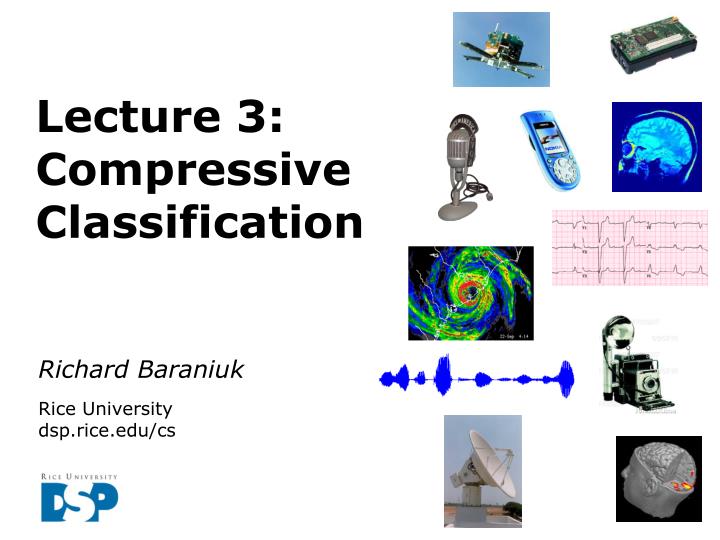
Lecture 3: Compressive Classification. Richard Baraniuk Rice University dsp.rice.edu/cs. Compressive Sampling. Signal Sparsity. large Gabor (TF) coefficients. wideband signal samples. Fourier matrix. Compressive Sampling. Random measurements. signal. measurements. sparse in basis.

E N D
Lecture 3: CompressiveClassification Richard Baraniuk Rice University dsp.rice.edu/cs
Signal Sparsity largeGabor (TF)coefficients widebandsignalsamples Fourier matrix
Compressive Sampling • Random measurements signal measurements sparsein basis
Compressive Sampling • Universality
Why Does It Work? (1) • Random projection not full rank, but stably embeds • sparse/compressible signal models (CS) • point clouds (JL) into lower dimensional space with high probability • Stable embedding: preserves structure • distances between points, angles between vectors, … provided M is large enough: Compressive Sampling K-sparsemodel K-dim planes
Why Does It Work? (2) • Random projection not full rank, but stably embeds • sparse/compressible signal models (CS) • point clouds (JL) into lower dimensional space with high probability • Stable embedding: preserves structure • distances between points, angles between vectors, … provided M is large enough: Johnson-Lindenstrauss Q points
Information Scalability • In many CS applications, full signal recovery may not be required • If we can reconstruct a signal from compressive measurements, then we should be able to perform other kinds of statistical signal processing: • detection • classification • estimation …
Classification of Signals in Noise • Observe one of Pknown signals in noise • Probability density function of the noiseex: zero mean, white Gaussian noise (AWGN) • Probability density function of signal >>> mean shifted to
Multiclass Likelihood Ratio Test (LRT) • Observe one of Pknown signals in noise • Classify according to: • AWGN: nearest-neighborclassification • Sufficient statistic:
Compressive LRT • Compressive observations: by the JL Lemmathese distancesare preserved • [Waagen et al 05, Davenport et al 06, Haupt et al 06]
Compressive LRT • Compressive observations: • If are normalized, these anglesare preserved
Performance of Compressive LRT • ROC curve for Neyman-Pearson detector (2 classes): • From JL lemma, for random orthoprojector • Thus • Penalty for compressive measurements: false alarm probability
Performance of Compressive LRT fewer measurements better SNR
Summary • If CS system is a random orthoprojector, then detection/classification problems in the signal space map into analogous problems in the measurement space • SNR penalty for compressive measurements • Note: Signal sparsity unexploited!
Matched Filter • In many applications, signals are transformedwith an unknown parameter; ex: translation • Elegant solution: matched filter Compute for all • Simultaneously: estimates parameterclassifies signal convolution of measurementwith template reversed in time
Compressive Matched Filter • Challenge: Extend matched filter concept to compressive measurements • GLRT: • GLRT approach extends to any case where each class can be parameterized with K parameters • If mapping from parameters to signal is well-behaved, then each class forms a manifold in
What is a Manifold? “Manifolds are a bit like pornography: hard to define, but you know one when you see one.” – S. Weinberger [Lee] • Locally Euclidean topological space • Roughly speaking: • a collection of mappings of open sets of RKglued together (“coordinate charts”) • can be an abstract space, not a subset of Euclidean space • e.g., SO3, Grassmannian • Typically for signal processing: • nonlinear K-dimensional “surface” in signal space RN
Examples • Circle in RN • parameter: angle • Chirp in RN • parameters: start frequency end frequency • Image appearance manifold • parameters: position of object, camera, lighting, etc.
Object Rotation Manifold each imageis a pointin RN K=1
Up/Down Left/Right Manifold [Tenenbaum, de Silva, Langford] K=2
Manifold Learning from Training Data • Translating disk parameters: left/right, up/down shift (K=2) • Generate training data by sampling from the manifold • “Learn” the structure of the manifold LaplacianEigenmaps ISOMAP HLLE R4096
Manifold Classification • Now suppose data is drawn from one of P possible manifolds: • AWGN: nearest manifold classification M1 M3 M2
Compressive Manifold Classification • Compressive observations: ?
Compressive Manifold Classification • Compressive observations: • Good news: structure of smoothmanifolds is preserved by randomprojection provided • distances, geodesic distances, angles, … [Wakin et al, 06, Haupt et al 07]
Stable Manifold Embedding Theorem: Let F½RN be a compact K-dimensional manifold with • condition number 1/t (curvature, self-avoiding) • volume V Let F be a random MxN orthoprojector with Then with probability at least 1-r, the following statement holds: For every pair x,y2F • [Wakin et al 06, Haupt et al 07]
Stable Manifold Embedding • Theorem tells us that random projectionspreserve smooth manifold • dimensionality • ambient distances • geodesic distances • local angles • topology • local neighborhoods • Volume • Also there exists extension to some kinds of non-smooth manifolds
Manifold Learning from Compressive Measurements LaplacianEigenmaps ISOMAP HLLE R4096 RM M=15 M=15 M=20
Multiple Manifold Embedding Corollary: Let M1, … ,MP½RN be compact K-dimensional manifolds with • condition number 1/t (curvature, self-avoiding) • volume V • min dist(Mj,Mk) > (can be relaxed) Let F be a random MxN orthoprojector with Then with probability at least 1-r, the following statement holds: For every pair x,y 2 Mj
Compressive Manifold Classification • Compressive observations: • Good news: structure of smoothmanifolds is preserved by randomprojection provided • distances, geodesic distances, angles, … [Wakin et al, 06, Haupt et al 07]
Smashed Filter • Compressive manifold classification with GLRT • nearest-manifold classifier based on manifolds M1 M3 M2 M1 M3 M2 [Davenport et al 06, Healy and Rohode 07]
Smashed Filter – Experiments • 3 image classes: tank, school bus, SUV • N = 65,536 pixels • Imaged using single-pixel CS camera with • unknown shift • unknown rotation
Smashed Filter – Unknown Position • Object shifted at random (K=2 manifold) • Noise added to measurements • Goal: identify most likely position for each image class identify most likely class using nearest-neighbor test more noise classification rate (%) avg. shift estimate error more noise number of measurements M number of measurements M
Smashed Filter – Unknown Rotation • Object rotated each 10o • Goals: identify most likely rotation for each image class identify most likely class using nearest-neighbor test • Perfect classification with as few as 6 measurements • Good estimates of rotation with under 10 measurements avg. rot. est. error number of measurements M
Summary • Compressive measurementsareinformation scalable reconstruction > estimation > classification > detection • Random projections preserve structure of smooth manifolds (analogous to sparse signals) • Smashed filter: dimension-reduced GLRT for parametrically transformed signals • exploits compressive measurements and manifold structure • broadly applicable: targets do not have to have sparse representation in any basis • effective for detection/classification
Open Issues • Compressive classification does not exploit sparse signal structure to improve performance • Non-smooth manifolds and local minima in GLRT • one approach: multiscale random projections • Experiments with real data
Some References • R. G. Baraniuk, M. Davenport, R. DeVore, M. Wakin, “A simple proof of the restricted isometry property for random matrices,” to appear in Constructive Approximation, 2007. • R. G. Baraniuk and M. Wakin, “Random projections of smooth manifolds,” 2006; see also ICASSP 2006. • M. Davenport, M. Duarte, M. Wakin, J. Laska, D. Takhar, K. Kelly, R. G. Baraniuk, “The smashed filter for compressive classification and target recognition,” Proc. of Computational Imaging V at SPIE Electronic Imaging, San Jose, California, January 2007. • M. Wakin, D. Donoho, H. Choi, R. G. Baraniuk. “The multiscale structure of non-differentiable image manifolds,” Proc. Wavelets XI at SPIE Optics and Photonics, 2005. • J. Haupt, R. Castro, R. Nowak, G. Fudge, A. Yeh, “Compressive sampling for signal classification,” Proc. Asilomar Conference on Signals, Systems, and Computers, 2006. • D. Healy, G. Rohode, “Fast global image registration using random projections, 2007. for more, see dsp.rice.edu/cs