Download
1 / 46
460 likes | 625 Views
The relativistic time-dependent Aharonov-Bohm effect in two spatial dimensions. Athan Petridis Zachary Kertzman Drake University. The Aharonov-Bohm effect. The charged fermions interact directly with the e/m 4-potential, NOT the electric or magnetic fields.

E N D
The relativistic time-dependent Aharonov-Bohm effect in two spatial dimensions Athan Petridis Zachary Kertzman Drake University
The Aharonov-Bohm effect • The charged fermions interact directly with the e/m 4-potential, NOT the electric or magnetic fields. • Around an non-penetrable solenoid spinors diffract acquiring an extra phase. • Difficult to directly, experimentally confirm that it is not due to residual fields. • It is used by interferometry experiments. • Nanosecond pulse electron sources available.
The Dirac Equation • Relativistic quantum equation for spin-1/2 fermions, which are described by a 4-dimentional spinor Ψ. • Including an external scalar potential, V:
The Numerical Algorithm • The staggered leap-frog algorithm is applied in a spatial grid of bin-size Δx (in 1 dim) and with time step Δt: • The spatial derivatives are computed symmetrically. • Reflecting boundary conditions are applied on a very large grid (running stops before reflections occur if necessary). • Works well on a PC, using dynamic memory allocation.
Stability of the Algorithm • Use the norm as measure • The stability region is (d = spatial grid bin, Δt = time step) • Obtained via a standard stability analysis usingplane waves (for large component) probability 1 time
1D Free Electron Propagation • The initial spinor is (N = normalization factor, m =1): • The probability density ρ=Ψ†Ψ at t=0 is Gaussian (s.d.=σ0). • As σ0→∞,Ψ becomes a positive energy plane wave, which for p=0 is a spin +1/2 eigenstate. • ρ(x,t) is shown next for σ0=1. The method is stable. The accuracy is of order 10-10 per bin (Δx=0.01, Δt=0.001).
Position Expectation Value • <x> vs time after subtraction of the drift velocity (red: σ0 = 0.5, p = 0.01; green: σ0 = 0.5, p=1.37; blue: σ0=1, p=0.01, purple: σ0 =1.5, p=1.0). • High-frequency (~2E) oscillations are observed (Zitterbewegung). • The effect has a non-linear dependence on σ0 and is maximized when 2 σ0 = λc (Compton wavelength) for given p. It increases with p.
Standard Deviation • Standard deviation of the probability density, σ, vs time (red: σ0 = 0.5, p = 0; green: σ0 = 0.5, p=1.0; blue: σ0 = 1.0, p = 0; purple: σ0 = 1.0, p = 1.0; light blue: σ0 = 1.5, p = 0; yellow: σ0 = 1.5, p = 1.0). • High-frequency oscillations are more pronounced as p increases and die out with time. • σ increases faster at lower p.
Spin, z-component • Expectation value of the z-component of the spin (perpendicular to the propagation direction) (red: σ0 = 0.5, p = 0.01; green: σ0 = 0.5, p = 1.37; blue: σ0 = 1.0, p = 0.01; purple: σ0 = 4.0, p = 0.0). • The high-frequency oscillations die out with time and are maximized at 2σ0 = λc. • Results agree with J. W. Braun, Q. Su, and R. Grobe, Phys. Rev. A59, 604 (1999).
Decay and Survival Probability • A decaying fermionic system can be described as a Dirac spinor initially set inside a potential well that tunnels through the potential walls. • Introduce constant potential: V(x). • In a given reference frame, the survival probability of the system is defined as
Finite Square Well Potential • The width, 2a, is set equal to 2 σ0 with σ0 = λc = 1.0. • Pinvs time (p = 0) for V = 0.1 (red), 1.0 (green), 1.5 (blue), and 2.0 (purple) [A] and V = 0.1, p = 0.01 (red), V = 2.2, p = 0.01 (green), V = 0.9, p = 0.1 (blue) and V = 2.2, p = 0.1 (purple) [B]. • Pin decays non-exponentially performing oscillations. This has also been observed in non-relativistic decays. • The relativistic case includes a sudden increase in Pin for V > 1 due to Klein-paradox. The effect of p is small. A B
Strong solenoid + dipole field • Minimal substitution: • Infinite solenoid vector potential (r >R): • Dipole (residual) vector potential (r>R): • Cylindrical electric potential V=const. (r<R) • A0=0.88, B0=A0/10, k=1.134, σ0= 5, R=4
Weak solenoid + dipole field • Same type of potential but weaker. • A0=0.01, B0=A0/10, k=1.134, σ0= 5, R=4. • The wavefunction diffracts.
Comparison: with/out dipole • Results without the dipole do not differ much visually from those with dipole. • For a strong field the difference is a fraction of a percept per point and for a weak field is of order one part in a million. • The difference has azimuthal asymmetry and is time-dependent.
Spin with/out dipole • The same observations can be made for the z- component of the spin distribution. • The difference is even more subtle.
Quantum Ring (Gaussian) • A “solid” ring of size comparable to the correlation length (spread, s.d.) of the initial spinor surrounds the solenoid. • An initial Gaussian spinor inside the ring spreads around the ring radially and azimuthally.
Quantum Ring (eigenfunction) • The initial spinor is an azimuthal eigenfunction. It spreads only radially. • In the presence of an A-field it is “turned” around. The energy distribution does not change. • The phase of the large component characteristically changes in the presence of the magnetic potential.
Evolved large component phase difference between field and no-field cases
Perspectives • Coupled two-fermion systems. propagating in medium are studied. • Dynamic mass renormalization due to self-interaction is studied (interleaved Maxwell’s equations also used). • Strong interactions will be introduced.