Download
1 / 22
220 likes | 315 Views
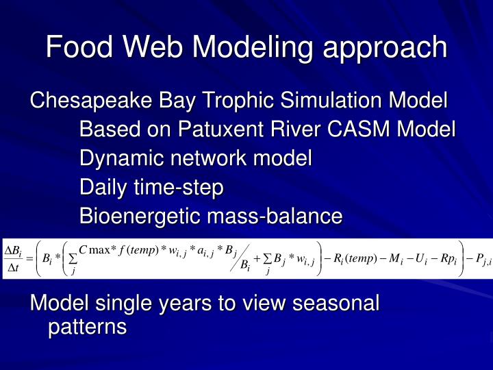
Food Web Modeling approach. Chesapeake Bay Trophic Simulation Model Based on Patuxent River CASM Model Dynamic network model Daily time-step Bioenergetic mass-balance Model single years to view seasonal patterns. Modeling Consumption. C max – Maximum Consumption Rate (g/g/d)

E N D
Food Web Modeling approach Chesapeake Bay Trophic Simulation Model Based on Patuxent River CASM Model Dynamic network model Daily time-step Bioenergetic mass-balance Model single years to view seasonal patterns
Modeling Consumption Cmax – Maximum Consumption Rate (g/g/d) wi,j – Preference of consumer i for prey j ai,j – assimilation efficiency of consumer i eating prey j f(t) – temperature adjustment of consumption Consumption follows seasonal patterns in both composition and rate
Modeling Energetic Costs and Mortality Rmax – maximum respiratory costs (g/g/d) U – Excretory losses SDA – Costs of consumption f(t) – Temperature adjustment of respiration rsp(i,t) – Consumer and season specific costs of egg production m(i) – Consumer specific natural mortality
Model Groups • 6 producer groups (phytoplankton by size) < 2 um, 2-4 um,. 4-10 um, 10-50 um, 50-100 um, > 100 um • 14 Consumer groups in seven categories zooplankton, gelatinous zooplankton, pelagic bacteria, pelagic forage fish, benthic invertebrates, benthic bacteria, benthic omnivorous fishes • 3 larval sub-pools bay anchovy, ctenophores, oysters
Main bay Model – Mesohaline Baywide average Tributary Model – Patuxent River Project Objectives
Larval Pools Pelagic Prey Fish Oyster Larvae Bay Anchovy Anchovy Larvae Ctenophore Larvae Atlantic Menhaden Gelatinous Zooplankton Zooplankton Sea Nettles Ctenophores Acartia tonsa Phytoplankton Microzoopnktn Non reef fish < 2 microns Pelagic Bacteria Benthic Reef-assoc. fish 2-4 microns HNAN 4-10 microns Oysters 10-50 mic On-reef inverts 50-100 mic Off-reef inverts > 100 microns Benthic Bacteria N P S DOC POC Detrital Pools
Pelagic Prey Fish Bay Anchovy Atlantic menhaden Gelatinous Zooplankton Sea Nettles Ctenophores Acartia tonsa Phytoplankton Microzoopnktn < 2 microns Zooplankton 2-4 microns “Lost” 4-10 microns Benthic Planktivores 10-50 mic 50-100 mic Oysters > 100 microns Detrital Pools
Bay Anchovy They were bigger in Oct
Modeling Oyster Recovery • Modeled 10X, 25X, and 50X scenarios • Assume threshold relationship between oysters and sea nettles • Assume linear relationship between oyster density, reef-associated fish, and on-reef invertebrates • Assume no relationship between oyster density and off-reef invertebrates Ex. 10X oysters = 10X on-reef inverts, 10X RAF, 20X SN
Phytoplankton Biomass Reduction Water quality model output from Noel and Cerco 2005 Table 1 - MD output