Download
1 / 35
430 likes | 756 Views
OC 430/530: Sverdrup circulation and Western Boundary Currents Nov 23, 2009. Finish geostrophy Barotropic and baroclinic pressure gradients Practical application of the geostrophic method Examples of the geostrophic method Limitations of the geostrophic method

E N D
OC 430/530: Sverdrup circulation and Western Boundary Currents Nov 23, 2009 • Finish geostrophy • Barotropic and baroclinic pressure gradients • Practical application of the geostrophic method • Examples of the geostrophic method • Limitations of the geostrophic method • Why do we still use the geostrophic method? • Review Ekman theory • wind-driven ocean circulation: Ekman + geostrophy = Sverdrup’s theory • Sverdrup’s method of solution • Wind forcing of the Sverdrup circulation: Wind stress curl = Ekman transport divergence • Closing the wind-driven circulation: Western boundary currents • Stommel’s solution: add bottom friction • Munk’s solution: add lateral friction (AH) • Conservation of potential vorticity and western boundary currents
A → acceleration B → pressure gradient force C → Coriolis force D → gravitational force E → other (friction, tidal, wind forcing, etc.) Compare to equations 7.12 a-c in Intro to PO+ + Intro to PO writes the material derivative out on the left hand side
Barotropic and baroclinic pressure gradients • Barotropic – pressure contours (isobars) parallel to density contours (isopycnals). Sea level changes and depth-averaged currents associated with barotropic pressure gradients • Baroclinic – pressure contours (isobars) inclined relative to density contours (isopycnals). Horizontal density gradients and depth-dependent flow result from baroclinic pressure gradients.
Geostrophic Balance Barotropic + baroclinic pressure gradient Drawn for northern hemisphere
For geostrophic estimates of velocity as a function of depth, we want to know the horizontal pressure gradients throughout the water column. In the ocean it is difficult to directly measure pressure relative to a known depth. However, we can estimate analogous quantities such as dynamic height or steric height (shown here) from the ocean density field. These quantities are relative to a (somewhat arbitrarily) specified level. (a) at 1500 m relative to 2000 m (b) at 0 m relative to 2000 m Dynamic height (m2 s-2) (or steric height multiplied by gravity) for the world ocean. Arrows indicate the direction of the implied movement of water. (Divide contour values by 10 to obtain approximate steric height in m.) Tomczak and Godfrey, 2001
Intro to deriving baroclinic pressure gradients from density measurements Consider a section through the ocean in which density (σt orσθ) varies horizontally and vertically. Given the isopycnal (constant density) contours and an assumed level of no motion (z0), the isobars (constant pressure) will be distributed as shown (a) due to the hydrostatic relation. If we consider surface zr, then pressure will be lowest at point A and higher east at point B (b). Similarly, the height of the pressure surface p1, will be lowest at point A and higher east and west (c). This pressure surface is directly analogous to the sea level change, p0. Tomczak and Godfrey, 2001
Practical application of the geostrophic method • In the previous calculations, we estimated the slope of an isobar (θ1, θ2, θ3) for one and two layer fluids and used this to estimate geostrophic velocity (vd). How do we estimate geostrophic velocity for realistic ocean density fields? • The technique still involves the vertical integration of the hydrostatic equation to get a quantity (geopotential anomaly) whose x and y derivatives approximate the pressure gradient • See section 10.4, Introduction to Physical Oceanography • Matlab programs from seawater toolbox available from the sea-mat website
Take the horizontal difference of geopotential anomaly (g multiplied by) the slope of the constant pressure surface P2
Notes on units ΔΦ is m2/s2 = J/kg f is s-1 L is m v is m/s! Some prefer to divide ΔΦ by g to get a quantity called steric height which is in meters and is directly analogous to sea level changes.
Left: Relative current calculated from hydrographic data collected south of Cape Cod in August 1982. The Gulf Stream is the fast current above 1000 decibars. The assumed depth of no motion is 2000 decibars. Right: Potential density σθacross the Gulf Stream along 63.66°W calculated from CTD data collected on 25–28 April 1986. The Gulf Stream is centered on the steeply sloping contours shallower than 1000m between 40° and 41°. The vertical scale is 425 times the horizontal scale. Note: The barotropic velocity is 0 here. All geostrophic velocity here is due to baroclinic pressure gradients
Mean geopotential anomaly of the Pacific Ocean relative to the 1,000 dbar surface based on 36,356 observations. Height is in geopotential centimeters. If the velocity at 1,000 dbar were zero, the map would be the surface topography of the Pacific. From Wyrtki (1974).
Data from expendable bathythermographs (XBT’s) with T/S relation derived from CTD’s • Red arrows indicate current meter data scaled such that arrow length corresponds to distance drifter would travel in one day • Blue tracks indicate drifters over one day. • Green arrows indicate wind speed and approximate Ekman velocity for slab-like surface boundary layer • Dynamic topography contoured in J/kg (m2/s2) • Dynamic topography does best in deep basin, less well near coast
Another example showing the performance of dynamic topography in a coastal region
Dynamic topography (geostrophic flow from pressure gradient) and egg production from Eucalanus in an upwelling filament Mackas (2005)
Limitations of the geostrophic method • Can only calculate currents relative to a level of no motion or known motion • Problems over shelf where there is no level of “no motion” • Density profiles affected by internal waves (short wavelength noise) • Assumes steady state, does not evolve in time • Problems at equator (f=0!) • Ignores friction, advection etc.
Why use the geostrophic method? • Still only practical method to yield data on internal pressure gradient • Combine with measured velocity, wind to get more complete picture of momentum balance • Hydrographic (density) data often acquired concurrently with biological, chemical data, matching its sampling
Ekman review In Ekman theory, the only friction considered is that due to downward transfer of momentum imparted by the surface wind stress
Ekman (1905) Ekman Transport: Due to wind and the Earth’s rotation Always to the right of the wind in Northern Hemisphere. No dependence on Az!
Geostrophic balance Although we haven’t done so, one could vertically integrate the solution to these equations and obtained a vertically-integrated geostrophic transport analogous to the Ekman transport
Ekman+ Geostrophy We can add Ekman transport and geostrophy since are both linear approximations (in that they do not involve terms with u2 or v2) of the conservation of momentum.
Sverdrup’s solution • Don’t worry about the vertical structure of flow, integrate vertically. This is similar in spirit to the integrated Ekman transport. • Eliminate pressure gradients by taking the y derivative of the x-momentum equation, the x-derivative of the y-momentum equation and subtracting the x-momentum from y-momentum (i.e., the curl) • Intro to PO has comments about Sverdrup solution (Chap 11) which you should read
Sverdrup’s solution My is mass transport in the y direction (north-south), β is the latitudinal variation of the Coriolis acceleration, f, τx and τy are east-west and north-south wind stresses, β = 2Ωcosφ/R Since wind stress is mostly zonal, neglect ∂τy/∂x Equation of continuity, Mx is mass transport in x direction And implies Δx is the distance from the eastern boundary, Ω is earth’s rotation rate, φ is latitude, R is radius of earth
Sverdrup circulation for simplified wind stress Simple, idealized wind stress My, Mx curl E W
y x What is sign of the wind stress curl (vorticity) of each of the sets of wind arrows below? A C D E B curl
Wind stress curl = Ekman transport divergence Negative wind stress curl: convergence and downwelling (positive curl would have divergence and upwelling) No wind stress curl: no divergence Tomczak and Godfrey (2003)
Ekman transport divergence/convergence can be caused by 3 basic mechanisms • wind stress curl (A,B,C) – Sverdrup transport • a coastal boundary (E) – upwelling and eastern boundary currents • the change in the sign of the Coriolis parameter at the equator (D) – equatorial upwelling and the equatorial current Black arrows are wind stress, green arrows are Ekman transport Tomczak and Godfrey (2003)
Worldwide distribution of wind stress curl/ffrom ship-based climatology Annual mean distribution of curl(τ /f), or Ekman pumping, (10-3 kg m2 s-1). Positive numbers indicate upwelling. In the equatorial region (2°N - 2°S, shaded) curl(τ/f) is not defined; the distribution in this region is inferred and is not quantitative. Tomczak and Godfrey (2003)
The difference between this slide and the previous one is that wind stress curl is not divided by f here curl Global 4-year averages (August 1999–July 2003) of the curl of the surface wind stress over the world ocean computed from 25-km-resolution wind measurements by the QuikSCAT scatterometer. Chelton et al. (2004)
Depth-integrated Sverdrup transport applied globally using the wind stress from Hellerman and Rosenstein (1983). Contour interval is 10 Sverdrups. After Tomczak and Godfrey 1 Sverdrup = 106 m3/s (not an SI unit but commonly used in oceanography) Introduction to Physical Oceanography
Sverdrup’s solution has a problem • Since there’s no friction other than wind stress, it keeps increasing to the west. Eventually you run out of room and need to account for the western boundary somehow. • In the previous slide, a western boundary was tacked on to account for the continuity equation, but no physical explanation was given.
Western Boundary currents: Stommel’s solution linearized bottom stress (new!) Simple, idealized wind stress (like Sverdrup) Stream function for flow in a basin as calculated by Stommel (1948). Left: Flow for non-rotating basin or flow for a basin with constant rotation. Right: Flow when rotation varies linearly with y. Introduction to Physical Oceanography
Western Boundary currents: Munk’s solution Added lateral friction (AH) Left: Mean wind stress wind stress curl. Upper Right: The mass transport stream function using observed wind stress. Contour interval is 10 Sverdrups. Lower Right: North-South component of the mass transport. After Munk (1950). Introduction to Physical Oceanography
Sverdrup, Stommel and Munk compared All start with geostrophy Sverdrup: only included wind stress at z = 0 Stommel: added bottom friction at z = -D (and kept the wind stress) Munk: dropped the bottom friction, added lateral friction (and kept the wind stress)
The conservation of potential vorticity and Western boundary currents Conservation of potential vorticity is a form of conservation of angular momentum. For Stommel’s model H is constant (flat bottom) and ζ + f is constant. ζ is the relative vorticity imparted by wind stress curl or friction at the western boundary constant