Download
1 / 16
170 likes | 382 Views
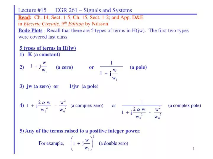
Lecture #15 EGR 261 – Signals and Systems. Read : Ch. 14, Sect. 1-5; Ch. 15, Sect. 1-2; and App. D&E in Electric Circuits, 9 th Edition by Nilsson. Bode Plots - Recall that there are 5 types of terms in H(jw). The first two types were covered last class. 5 types of terms in H(jw)

E N D
Lecture #15 EGR 261 – Signals and Systems Read: Ch. 14, Sect. 1-5; Ch. 15, Sect. 1-2; and App. D&E in Electric Circuits, 9th Edition by Nilsson Bode Plots - Recall that there are 5 types of terms in H(jw). The first two types were covered last class. 5 types of terms in H(jw) 1) K (a constant) 2) (a zero) or (a pole) 3) jw (a zero) or 1/jw (a pole) 4) 5) Any of the terms raised to a positive integer power.
Lecture #15 EGR 261 – Signals and Systems 1. Constant term in H(jw) If H(jw) = K = K/0 Then LM = 20log(K) and (w) = 0 , so the LM and phase responses are:
Lecture #15 EGR 261 – Signals and Systems 2A) term in H(jw) (a zero) 2B) term in H(jw) (a pole)
Lecture #15 EGR 261 – Signals and Systems Example: (from last class) Sketch the Bode LM and phase plots for:
Lecture #15 EGR 261 – Signals and Systems (End of review) Example: Sketch the LM and phase plots on the 4-cycle semi-log graph paper shown below for the following transfer function. (Pass out 2 sheets of graph paper.) Log-magnitude (LM) plot:
Lecture #15 EGR 261 – Signals and Systems Example: (continued) Phase plot:
Lecture #15 EGR 261 – Signals and Systems 3A) jw term in H(jw) If H(jw) = jw = w/90 Then LM = 20log(w) and (w) = 90 Calculate 20log(w) for several values of w to show that the graph is a straight line for all frequency with a slope of 20dB/dec (or 6dB/oct). The LM and phase for H(jw) = jw are shown below. • So a jw (zero) term in H(jw) adds an upward slope of +20dB/dec (or +6dB/oct) to the LM plot. • And a jw (zero) term in H(jw) adds a constant 90 to the phase plot.
Lecture #15 EGR 261 – Signals and Systems 3B) 1/(jw) term in H(jw) If H(jw) = 1/(jw) = (1/w)/-90 Then LM = 20log(1/w) = -20log(w) and (w) = -90 A few calculations could easily show that the graph of 20log(1/w)is a straight line for all frequency with a slope of -20dB/dec (or -6dB/oct). The LM and phase for H(jw) = 1/(jw) are shown below. • So a 1/(jw) (pole) term in H(jw) adds a downward slope of -20dB/dec (or -6dB/oct) to the LM plot. • And a 1/(jw) (pole) term in H(jw) adds a constant -90 to the phase plot.
Lecture #15 EGR 261 – Signals and Systems Example: Sketch the LM and phase plots for the following transfer function.
Lecture #15 EGR 261 – Signals and Systems Example: Sketch the LM and phase plots for the following transfer function.
Lecture #15 EGR 261 – Signals and Systems Calculation of exact points to check Bode Plots Evaluating H(jw) at a particular value of w is helpful to check Bode Plots. An example is shown below.
Lecture #15 EGR 261 – Signals and Systems Example: Evaluate the H(jw) on the last page at w = 500 rad/s and w = 8000 rad/s. Compare the values with the Bode plots. Do they appear to be correct?
Lecture #15 EGR 261 – Signals and Systems 5. Poles and zeros raised to an integer power in H(s) In the last class it was demonstrated that terms in H(jw) are additive. Therefore, a double terms (such as a pole or zero that is squared) simply acts like two terms, a triple term acts like three terms, etc. Illustration: Show that (1 + jw/w1)N results in the following responses: LM plot: Has a 0dB contribution before its break frequency Will increase at a rate of 20NdB/dec after the break There will be an error of 3NdB at the break between the Bode straight-line approximation and the exact LM Phase plot: Has a 0 degree contribution until 1 decade before its break frequency Will increase at a rate of 45Ndeg/dec for two decades (from 0.1w1 to 10w1). The total final phase contribution will be 90N degrees.
Lecture #15 EGR 261 – Signals and Systems So (1 + jw/w1)N results in the following responses:
Lecture #15 EGR 261 – Signals and Systems Example: Sketch the LM plot for the following transfer function.
Lecture #15 EGR 261 – Signals and Systems Generating LM and phase plots using Excel and MathCAD: Refer to the handout entitled “Frequency Response” which includes detailed examples of creating LM and phase plots using Excel and MathCAD. Generating LM and phase plots using ORCAD: Refer to the handout entitled “PSPICE Example: Frequency Response (Log-Magnitude and Phase)” which includes a detailed example of creating LM and phase plots using ORCAD.


![K 1 = [HCO 3 - ] [H + ]](https://cdn1.slideserve.com/3309135/slide1-dt.jpg)