Download
1 / 62
620 likes | 626 Views
University of G iro na. Computer Vision and Robotics. Pattern Projection Techniques. Presentation outline. 1.- A Survey of Pattern Projection Techniques Introduction and some classifications Pattern Projection Techniques Experimental results Conclusions & guidelines

E N D
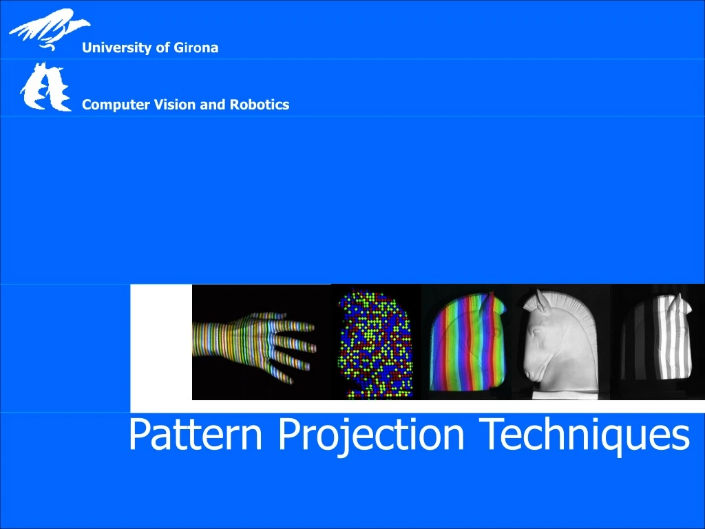
University of Girona Computer Vision and Robotics Pattern Projection Techniques
Presentation outline 1.- A Survey of Pattern Projection Techniques • Introduction and some classifications • Pattern Projection Techniques • Experimental results • Conclusions & guidelines 2.- An Optimised one-shot technique • Optimal pattern • A new coding strategy • Implementation design • Experimental results • Conclusions
Presentation outline Formació Introduction 1.- A Survey of Pattern Projection Techniques • Introduction and some classifications • Pattern Projection Techniques • Time Multiplexing • Spatial Codification • Direct Codification • Experimental results • Conclusions & guidelines Classification Experiments Conclusions
The challenge of Computer Vision INTERPRETATION Interpretation KNOWLEDGE DATA BASE BASE Level Introduction Shape acquisition Encoding/ decoding SCENE FUSION TRACKING DESCRIPTION Description Level SCENE SHAPE LOCALIZATION ANALYSIS IDENTIFICATION SEGMENTATION SHAPE ACQUISITION Classification TEXTURE FEATURE Image Processing ANALYSIS EXTRACTION High Level MOVEMENT DETECTION EDGE IMAGE RESTORATION RESTORATION Experiments EDGE FILTERING THINNING EDGE Image Processing Conclusions DETECTION Low Level THRESHOLDING COLOUR COMPENSATION GRADIENTS RE-HISTOGRAMATION A/D Image Acquisition COLOUR Level SEPARATION SENSOR
Shape Acquisition Techniques Shape acquisition techniques Introduction Shape acquisition Encoding/ decoding Non-contact Contact Reflective Transmissive Non-destructive Destructive Non-optical ... Slicing Classification CMM Jointed arms Microwave radar Sonar Optical Active Experiments Passive Conclusions Shape from X Interferometry (Coded) Structured light Moire Holography Motion Stereo Shading Silhouettes Texture Source: Brian Curless
Introduction: passive stereovision • Correspondence problem • geometric constraints • search along epipolar lines • 3D reconstruction of matched pairs by triangulation Introduction Shape acquisition Stereovision Encoding/ decoding Classification Experiments Sub-pixel matching Conclusions
Direct order Inverse order Introduction: passive stereovision • Arrange correspondence points • Ordered Projections • Projections bad order • Occlusions • Points without homologue Introduction Shape acquisition Stereovision Encoding/ decoding Classification Experiments Sub-pixel matching Conclusions Surface occlusion Point without homologue
Y M w X w Z w Z’ Z C’ C f’ m’ f Y’ I O’ m O Y I’ X X’ Captured Image Captured Image Introduction: passive stereovision • We need at least two cameras. • A 3D object point has three unknown co-ordinates. • Each 2D image point gives two equations. • Only a single component of the second point is needed. Introduction Shape acquisition Stereovision Encoding/ decoding Classification Experiments Sub-pixel matching Conclusions
Introduction: active stereo (coded structured light) Introduction Shape acquisition Stereovision Encoding/ decoding • One of the cameras is replaced by a light emitter • Correspondence problem is solved by searching the pattern in the camera image (pattern decoding) Classification Experiments Sub-pixel matching Conclusions
Coded Structured Light • The correspondence problem is reduced : • The matching between the projected pattern and the captured one can be uniquely solved codifying the pattern. Introduction Shape acquisition Encoding/ decoding • Single dot : • No correspondence problem. • Scanning both axis. • Single slit : • No correspondence problem. • Scanning the axis orthogonal to the slit. • Stripe patterns : • No scanning. • Correspondence problem among slits. • Grid, multiple dots : • No scanning. • Correspondence problem among all the imaged features (points, dots, segments,…). Classification Experiments Conclusions
Pattern encoding/decoding (I) Introduction Shape acquisition Encoding/ decoding • A pattern is encodedwhen after projecting it onto a surface, a set of regions of the observed projection can be easily matched with the original pattern. Example: pattern with two-encoded-columns • The process of matching an image region with its corresponding pattern region is known as pattern decoding similar to searching correspondences • Decoding a projected pattern allows a large set of correspondences to be easily found thanks to the a priori knowledge of the light pattern Object scene Pixels in red and yellow are directly matched with the pattern columns Codification using colors Classification Experiments Conclusions
Pattern encoding/decoding (II) Introduction Shape acquisition Encoding/ decoding • Two ways of encoding the correspondences: single and double axis codification it determines how the triangulation is calculated • Decoding the pattern means locating points in the camera image whose corresponding point in the projector pattern is a priori known Single-axis encoding Double-axis encoding Triangulation by line-to-plane intersection Triangulation by line-to-line intersection Classification Encoded Axis Experiments Encoded Axis Conclusions
Coded structured light patterns: a classification proposal AXIS CODIFICATION SCENE APPLICABILITY Introduction • Static Scenes • - Projection of a set of patterns. • Single Axis • - Row-coded patterns • - Column-coded patterns Classification Time-multiplexing Spatial codification Direct codification • Moving Scenes • - Projection of a unique pattern. • Both Axis PIXEL DEPTH CODING STRATEGY Experiments • Periodical • - The codification of the tokens • is repeated periodically. • Binary • Grey Levels • Colour Conclusions • Absolute • - Each token is uniquely encoded
Coded structured light patterns: a classification proposal Introduction Classification Time-multiplexing Spatial codification Direct codification Experiments Conclusions
Time-multiplexing Example: 3 binary-encoded patterns which allows the measuring surface to be divided in 8 sub-regions Introduction • The time-multiplexing paradigm consists of projecting a series of light patterns so that every encoded point is identified with the sequence of intensities that receives • The most common structure of the patterns is a sequence of stripes increasing its length by the time single-axis encoding • Advantages: • high resolution a lot of 3D points • High accuracy (order of m) • Robustness against colorful objects (using binary patterns) • Drawbacks: • Static objects only • Large number of patterns High computing time Classification Time-multiplexing Spatial codification Direct codification Projected over time Pattern 3 Experiments Pattern 2 Conclusions Pattern 1
Time-multiplexing: Binary codes (I) • Every encoded point is identified by the sequence of intensities that receives • n patterns must be projected in order to encode 2n stripes Introduction Example: 7 binary patterns proposed by Posdamer & Altschuler Classification Time-multiplexing Spatial codification Direct codification Projected over time … Experiments Pattern 3 Pattern 2 Conclusions Pattern 1 Codeword of this píxel: 1010010 identifies the corresponding pattern stripe
Time-multiplexing: binary codes (II) • Coding redundancy: every edge between adjacent stripes can be decoded by the sequence at its left or at its right Introduction Formació Classification Time-multiplexing Spatial codification Direct codification Experiments Conclusions
Time-multiplexing: n-ary codes (I) • n-ary codes reduce the number of patterns by increasing the number of projected intensities (grey levels/colours) increases the basis of the code • The number of patterns, the number of grey levels or colours and the number of encoded stripes are strongly related fixing two of these parameters the reamaining one is obtained Introduction Classification Time-multiplexing Spatial codification Direct codification Using a binary code, 6 patterns are necessary to encode 64 stripes Experiments Conclusions Using a 4-ary code, 3 patterns are used to encode 64 stripes (Horn & Kiryati)
Time-multiplexing: n-ary codes (II) Introduction • n-ary codes reduce the number of patterns by increasing the number of projected intensities (grey levels/colours) Classification Time-multiplexing Spatial codification Direct codification Experiments Conclusions
Time-multiplexing: Gray code + Phase shifting (I) Introduction • A sequence of binary patterns (Gray encoded) are projected in order to divide the object in regions Example: three binary patterns divide the object in 8 regions Classification Time-multiplexing Spatial codification Direct codification Without the binary patterns we would not be able to distinguish among all the projected slits • An additional periodical pattern is projected • The periodical pattern is projected several times by shifting it in one direction in order to increase the resolution of the system similar to a laser scanner Experiments Conclusions Every slit always falls in the same region Gühring’s line-shift technique
Time-multiplexing: Gray code + Phase shifting (II) • A periodical pattern is shifted and projected several times in order to increase the resolution of the measurements • The Gray encoded patterns permit to differentiate among all the periods of the shifted pattern Introduction Classification Time-multiplexing Spatial codification Direct codification Experiments Conclusions
Time-multiplexing: hybrid methods (I) • In order to decode an illuminated point it is necessary to observe not only the sequence of intensities received by such a point but also the intensities of few (normally 2) adjacent points • The number of projected patterns reduces thanks to the spatial information that is taken into account • The redundancy on the binary codification • is eliminated Introduction Formació Classification Time-multiplexing Spatial codification Direct codification 1 0 Pattern 1 Hall-Holt and Rusinkiewicz technique: 4 patterns with 111 binary stripes Edges encoding: 4x2 bits (every adjacent stripe is a bit) 1 1 Pattern 2 Experiments 0 1 Pattern 3 Conclusions 0 1 Pattern 4 Edge codeword: 10110101
Time-multiplexing: hybrid methods (II) Introduction Classification Time-multiplexing Spatial codification Direct codification Experiments Conclusions
Spatial Codification Introduction • Spatial codification paradigm encodes a set of points with the information contained in a neighborhood (called window) around them • The codification is condensed in a unique pattern instead of multiplexing it along time • The size of the neighborhood (window size) is proportional to the number of encoded points and inversely proportional to the number of used colors • The aim of these techniques is to obtain a one-shot measurement system moving objects can be measured Classification Time-multiplexing Spatialcodification Direct codification • Drawbacks: • Discontinuities on the object surface can produce erroneous window decoding (occlusions problem) • The higher the number of used colours, the more difficult to correctly identify them when measuring non-neutral coloured surfaces Experiments • Advantages: • Moving objects supported • Possibility to condense the codification into a unique pattern Conclusions
Spatial codification: non-formal codification (I) • The first group of techniques that appeared used codification schemes with no mathematical formulation. • Drawbacks: • the codification is not optimal and often produces ambiguities since different regions of the pattern are identical • the structure of the pattern is too complex for a good image processing Introduction Classification Time-multiplexing Spatialcodification Direct codification Durdle et al. periodic pattern Experiments Conclusions Maruyama and Abe complex structure based on slits containing random cuts
Spatial codification: non-formal codification (II) Introduction Classification Time-multiplexing Spatialcodification Direct codification Experiments Conclusions
Spatial codification: De Bruijn sequences (I) • A De Bruijn sequence(orpseudorrandom sequence)of order m over an alphabet of n symbols is a circular string of length nm that contains every substring of length m exactly once (in this case the windows are unidimensional). • 1000010111101001 Introduction m=4 (window size) n=2 (alphabet symbols) Classification Time-multiplexing Spatialcodification Direct codification • Formulation: • Given P={1,2,...,p} set of colours. • We want to determine S={s1,s2,...sn} sequence of coloured slits. • Node: {ijk} Î • Number of nodes: p3 nodes. • Transition {ijk} Ù {rst} Þ j = r, k = s • The problem is reduced to obtain the path which visits all the nodes of the graph only once (a simple variation of the Salesman’s problem). • Backtracking based solution. • Deterministic and optimally solved by Griffin. m = 3 (window size) n = p (alphabet symbols) Experiments Conclusions
121 212 112 122 111 222 211 221 Spatial codification: De Bruijn sequences (II) Example: p = 2 Path: (111),(112),(122),(222),(221),(212),(121),(211). Slit colour sequence:111,2,2,2,1,2,1,1 Þ Maximum 10 slits. ‘1’ Red ‘2’ Green Introduction m = 3 n = 2 Classification Time-multiplexing Spatialcodification Direct codification Experiments Conclusions
Spatial codification: De Bruijn sequences (III) • The De Bruijn sequences are used to define coloured slit patterns (single axis codification) or grid patterns (double axis codification) • In order to decode a certain slit it is only necessary to identify one of the windows in which it belongs to Introduction Classification Time-multiplexing Spatialcodification Direct codification Experiments Conclusions Zhang et al.: 125 slits encoded with a De Bruijn sequence of 5 colors and window size of 3 slits Salvi et al.: grid of 2929 where a De Bruijn sequence of 3 colors and window size of 3 slits is used to encode the vertical and horizontal slits
Spatial codification: De Bruijn sequences (IV) Introduction Classification Time-multiplexing Spatialcodification Direct codification Experiments Conclusions
Spatial codification: M-arrays (I) • An m-array is the bidimensional extension of a De Bruijn sequence. Every window of wh units appears only once. The window size is related with the size of the m-array and the number of symbols used • 0 0 1 0 1 0 • 0 1 0 1 1 0 • 1 1 0 0 1 1 • 0 0 1 0 1 0 Introduction Classification Time-multiplexing Spatialcodification Direct codification Example: binary m-array of size 46 and window size of 22 Experiments Conclusions M-array proposed by Vuylsteke et al. Represented with shape primitives Morano et al. M-array represented with an array of coloured dots
Spatial codification: M-arrays (II) Introduction Classification Time-multiplexing Spatialcodification Direct codification Experiments Conclusions
Direct Codification • Every encoded pixel is identified by its own intensity/colour • Since the codification is usually condensed in a unique pattern, the spectrum of intensities/colours used is very large • Additional reference patterns must be projected in order to differentiate among all the projected intensities/colours: • Ambient lighting (black pattern) • Full illuminated (white pattern) • … • Advantages: • Reduced number of patterns • High resolution can be teorically achieved (all points are coded) • Drawbacks: • Very noisy in front of reflective properties of the objects, non-linearities in the camera spectral response and projector spectrum non-standard light emitters are required in order to projectsingle wave-lengths • Low accuracy (order of 1 mm) Introduction Classification Time-multiplexing Spatial codification Direct codification Experiments Conclusions
Direct codification: grey levels (I) • Every encoded point of the pattern is identified by its intensity level Introduction Classification Time-multiplexing Spatial codification Direct codification Every slit is identified by its own intensity Experiments Carrihill and Hummel Intensity Ratio Sensor: fade from black to white Conclusions • Every slit must be projected using a single wave-length • Cameras with large depth-per-pixel (about 11 bits) must be used in order to differentiate all the projected intensities Requirements to obtain high resolution
Direct codification: grey levels (II) Introduction Classification Time-multiplexing Spatial codification Direct codification Experiments Conclusions
Direct codification: Colour (I) Introduction • Every encoded point of the pattern is identified by its colour Classification Time-multiplexing Spatial codification Direct codification Tajima and Iwakawa rainbow pattern (the rainbow is generated with a source of white light passing through a crystal prism) T. Sato patterns capable of cancelling the object colour by projecting three shifted patterns (it can be implemented with an LCD projector if few colours are projected drawback: the pattern becomes periodic in order to maintain a good resolution) Experiments Conclusions
Direct codification: Colour (II) Introduction Classification Time-multiplexing Spatial codification Direct codification Experiments Conclusions
De Bruijn Gühring Experimental results Introduction Classification Experiments Conclusions
Conclusions Introduction Classification Experiments Conclusions Guidelines
Guidelines Introduction Classification Experiments Conclusions Guidelines
Presentation outline Introduction 2.- An Optimised one-shot technique • Typical one-shot patterns • Optimal pattern • A new coding strategy • Implementation design • Experimental results • Conclusions One-shot patterns Optimisation Coding strategy design Experiments Conclusions
Typical one-shot patterns De Bruijn codification Introduction Image by Li Zhang One-shot patterns Optimisation Stripe pattern Multi-slit pattern Grid pattern M-array codification Coding strategy design Experiments Checkerboard pattern Conclusions Array of shape primitives Array of dots
Best one-shot patterns Introduction One-shot patterns Optimisation Coding strategy design Experiments Conclusions
Optimising De Bruijn patterns: interesting features Introduction One-shot patterns Optimisation Coding strategy design Experiments Conclusions
Optimisation: maximising resolution Ideal pattern: the one which downsamples the projector resolution so that all the projected pixels are perceived in the camera image in fact only columns or rows must be identified in order to triangulate 3D points. Introduction One-shot patterns Optimisation Stripe patterns: achieve maximum resolution since they are formed by adjacent bands of pixels. Coding strategy design Multi-slit patterns: the maximum resolution is not achieved since black gaps are introduced between the slits Experiments Conclusions
Optimisation: maximising accuracy Ideal pattern: multi-slit patterns allow intensity peaks to be detected with precise sub-pixel accuracy Introduction One-shot patterns Multi-slit pattern Stripe pattern Optimisation RGB channels intensity profile of a row of the image Coding strategy Edge detection between stripes: need to find edges in the three RGB channels the location of the edges does not coincide design Experiments Conclusions Figure by Jens Gühring
Optimisation: minimising the window size and the number of colours Introduction One-shot patterns Optimisation Coding strategy design Experiments If both the number of colours and the window size are minimised the resolution decreases Conclusions
Optimising De Bruijn patterns: summary Introduction One-shot patterns Optimisation Coding strategy design Experiments Conclusions
Projected luminance profile intensity Horizontal scanline Perceived luminance profile intensity intensity Horizontal scanline Horizontal scanline A new hybrid pattern Combination of the advantages of stripe patterns and multi-slit patterns Introduction One-shot patterns Multi-slit pattern in the Luminance channel Stripe pattern in the RGB space Optimisation Coding strategy design Experiments Conclusions
The new coding strategy Example: n=4, m=3 Given n different values of Hue and a window size of length m 128 stripes Introduction One-shot patterns A pattern with 2nm stripes is defined with a square Luminance profile with alternating full-illuminated and half-illuminated stripes 32 stripes … 32 stripes Optimisation Coding strategy The pattern is divided in n periods so that all the full-illuminated stripes of every period share the same Hue design 16 coded stripes … 16 coded stripes The half-illuminated stripes of every period are coloured according to a De Bruijn sequence of order m-1 and the same n Hue values Experiments Conclusions