Interval Finite Elements as a Basis for Generalized Models of Uncertainty in Engineering Analysis

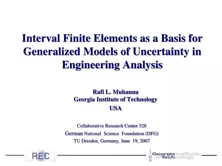
1. Interval Finite Elements as a Basis forGeneralized Models of Uncertainty inEngineering Analysis Rafi L. MuhannaGeorgia Institute of Technology USA Collaborative Research Center 528 German National Science Foundation (DFG) TU Dresden, Germany, June 19, 2007

2. Outline • Introduction • Interval Arithmetic • Interval Finite Elements • Element-By-Element • Examples • Conclusions

3. Outline • Introduction • Interval Arithmetic • Interval Finite Elements • Element-By-Element • Examples • Conclusions

4. Introduction- Uncertainty • Uncertainty is unavoidable in engineering system • structural mechanics entails uncertainties in material, geometry and load parameters (aleatory-epistemic) • Probabilistic approach is the traditional approach • requires sufficient information to validate the probabilistic model • criticism of the credibility of probabilistic approach when data is insufficient (Elishakoff, 1995; Ferson and Ginzburg, 1996; Möller and Beer, 2007)

5. Introduction- Interval Approach • Nonprobabilistic approach for uncertainty modeling when only range information (tolerance) is available • Represents an uncertain quantity by giving a range of possible values • How to define bounds on the possible ranges of uncertainty? • experimental data, measurements, statistical analysis, expert knowledge

6. Introduction- Why Interval? • Simple and elegant • Conforms to practical tolerance concept • Describes the uncertainty that can not be appropriately modeled by probabilistic approach • Computational basis for other uncertainty approaches (e.g., fuzzy set, random set, imprecise probability) • Provides guaranteed enclosures

7. Outline • Introduction • Interval Arithmetic • Interval Finite Elements • Element-By-Element • Examples • Conclusions

8. Interval arithmetic –Background • Archimedes (287 - 212 B.C.) •  circle of radius one has an area equal to 

9. r =1 r=1 Interval arithmetic –Background • Archimedes (287 - 212 B.C.) •  circle of radius one has an area equal to  •  = [3.14085, 3.14286]

10. Interval arithmetic –Background • Modern interval arithmetic • Physical constants or measurements g  [9.8045, 9.8082] • Representation of numbers  • Rounding errors   • R. E. Moore, E. Hansen , A. Neumaier, G. Alefed, J. Herzberger

11. Interval arithmetic Interval number represents a range of possible values within a closed set

12. Interval Operations Let x = [a, b]and y = [c, d]be two interval numbers 1. Addition x + y = [a, b] + [c, d] = [a + c, b + d] 2. Subtraction x y = [a, b]  [c, d] = [a d, b c] 3. Multiplication xy= [min(ac,ad,bc,bd),max(ac,ad,bc,bd)] 4. Division 1 / x = [1/b, 1/a]

13. Properties of Interval Arithmetic Let x, yand z be interval numbers 1. Commutative Law x + y = y + x xy = yx 2. Associative Law x + (y + z) = (x + y) + z x(yz) = (xy)z 3.Distributive Law does not always hold,but x(y + z)xy + xz

14. Sharp Results–Overestimation • The DEPENDENCY problem arises when one or several variables occur more than once in an interval expression • f(x) = x  x , x=[1, 2] • f(x) = [1  2, 2  1] = [1, 1]0 • f (x, y) = { f (x, y) =x y | x x, y  y} • f (x) = x (1 1) f (x) = 0 • f (x) = { f (x) =x x | x x}

15. Sharp Results–Overestimation • If a, band c are interval numbers, then: a (bc)abac • If we set a = [2, 2]; b = [1, 2]; c = [2, 1], we get a (b + c)= [2, 2]([1, 2] + [2, 1]) = [2, 2] [1, 3] =[6, 6] • However, ab + ac= [2, 2][1, 2] + [2, 2][2, 1] = [4, 4] + [4, 4]=[8, 8]

16. Sharp Results–Overestimation • Interval Vectors and Matrices • An interval matrix is such matrix that contains all real matrices whose elements are obtained from all possible values between the lower and upper bounds of its interval components

17. Sharp Results–Overestimation • Let a, b, c and d be independent variables, each with interval [1, 3]

18. Introduction Interval Arithmetic Interval Finite Elements Element-By-Element Examples Conclusions Outline

19. Finite Element Method (FEM) is a numerical method that provides approximate solutions to differential equations (ODE and PDE) Finite Elements

20. Mathematical model (validation) Discretization of the mathematical model into a computational framework Parameter uncertainty (loading, material properties) Rounding errors Finite Elements- Uncertainty& Errors

21. Interval Finite Elements Uncertain Data Materials Geometry Loads Interval Load Vector Interval Stiffness Matrix Element Level K U = F

22. = Interval element stiffness matrix B = Interval strain-displacement matrix C = Interval elasticity matrix F = [F1, ... Fi, ... Fn] = Interval element load vector (traction) Interval Finite Elements K U = F Ni = Shape function corresponding to the i-th DOF t = Surface traction

23. Follows conventional FEM Loads, geometry and material property are expressed as interval quantities System response is a function of the interval variables and therefore varies in an interval Computing the exact response range is proven NP-hard The problem is to estimate the bounds on the unknown exact response range based on the bounds of the parameters Interval Finite Elements (IFEM)

24. Combinatorial method (Muhanna and Mullen 1995, Rao and Berke 1997) Sensitivity analysis method (Pownuk 2004) Perturbation (Mc William 2000) Monte Carlo sampling method Need for alternative methods that achieve Rigorousness – guaranteed enclosure Accuracy – sharp enclosure Scalability – large scale problem Efficiency IFEM- Inner-Bound Methods

25. IFEM- Enclosure • Linear static finite element • Muhanna, Mullen, 1995, 1999, 2001,and Zhang 2004 • Popova 2003, and Kramer 2004 • Neumaier and Pownuk 2004 • Corliss, Foley, and Kearfott 2004 • Dynamic • Dessombz, 2000 • Free vibration-Buckling • Modares, Mullen 2004, and Billini and Muhanna 2005

26. Then iff Interval Finite Elements • Interval Linear System of Equations A x = b

27. 0.5 1.0 x1 S (A, b) Ssym(A, b) Ssym(A, b) P1 = (0.3,  0.6) P2 = (0.6,  0.6) P3 = (0.6,  0.3) P4 = (0.4,  0.4) 0.5 S (A, b) A–1b 1.0 x2 Interval Finite Elements P3 P4 P1 P2

28. Outline • Introduction • Interval Arithmetic • Interval Finite Elements • Element-By-Element • Examples • Conclusions

29. Naïve interval FEA • exact solution: u2 = [1.429, 1.579], u3 = [1.905, 2.105] • naïve solution: u2 = [－0.052, 3.052], u3 = [0.098, 3.902] • interval arithmetic assumes that all coefficients are independent • uncertainty in the response is severely overestimated (1900%)

30. Element-By-Element Element-By-Element (EBE) technique • elements are detached –no element coupling • structure stiffness matrix is block-diagonal (k1 ,…, kNe) • the size of the system is increased u = (u1, …, uNe)T • need to impose necessary constraints for compatibility and equilibrium Element-By-Element model

31. Element-By-Element

32. Element-By-Element • : • :

33. Constraints Impose necessary constraints for compatibility and equilibrium • Penalty method • Lagrange multiplier method Element-By-Element model

34. Constraints – penalty method

35. Constraints – Lagrange multiplier

36. Nodal load pb Load in EBE

37. For the interval equation Ax = b, preconditioning: RAx = Rb, R is the preconditioning matrix transform it into g(x*) = x*: R b –RA x0+ (I – RA) x*=x*, x = x*+x0 Theorem (Rump, 1990): for some interval vector x*, if g(x*)  int (x* ) then AHb  x*+x0 Iteration algorithm: No dependency handling Fixed point iteration

38. Fixed point iteration • , • ,

39. Convergence of fixed point • The algorithm converges if and only if • To minimize ρ(|G|): • : • 1

40. Stress calculation • Conventional method: • Present method:

41. Element nodal force calculation • Conventional method: • Present method:

42. Outline • Introduction • Interval Arithmetic • Interval Finite Elements • Element-By-Element • Examples • Conclusions

43. Numerical example • Examine the rigorousness, accuracy, scalability, and efficiency of the present method • Comparison with the alternative methods • the combinatorial method, sensitivity analysis method, and Monte Carlo sampling method • these alternative methods give inner estimation

44. Examples – Load Uncertainty • Four-bay forty-story frame

45. Examples – Load Uncertainty • Four-bay forty-story frame Loading A Loading C Loading B Loading D

46. Examples – Load Uncertainty • Four-bay forty-story frame Total number of floor load patterns 2160 = 1.46  1048 If one were able to calculate 10,000 patterns / s there has not been sufficient time since the creation of the universe(4-8)billion years ? to solve all load patterns for this simple structure Material A36, Beams W24 x 55, Columns W14 x 398 201 205 357 360 196 200 17.64 kN/m (1.2 kip/ft) 40@3.66 m = 146.3 m (480 ft) 10 6 201 204 5 1 1 5 14.63 m (48 ft)

47. Elements 1 2 3 Nodes 1 6 2 7 3 8 Combination solution Total number of required combinations = 1.461501637  1048 Interval Axial force (kN) [-2034.5, 185.7] [-2161.7, 0.0] [-2226.7, 0.0] solution Shear force (kN) [-5.1, 0.9] [-5.8, 5.0] [-5.0, 5.0] Moment (kN m) [-10.3, 4.5] [-15.3, 5.4] [-10.6, 9.3] [-17, 15.2] [-8.9, 8.9] [-16, 16] Examples – Load Uncertainty • Four-bay forty-story frame Four bay forty floor frame - Interval solutions for shear force and bending moment of first floor columns

48. Examples – Load Uncertainty 31 22 • Ten-bay truss A = 0.006 m2 E = 2.0 108 kPa F = [-4.28, 28.3] kN Fmin= -(0.062+0.139+0.113) 20= -4.28 kN Fmax= (0.464+0.309+0.258+0.192+0.128+0.064) 20 =28.3 kN 22 2 5 m 1 2 11 1 21 13 12 20 21 20 kN 20 kN 20 kN 20 kN 20 kN 20 kN 20 kN 20 kN 20 kN 10 @ 4 = 40 m 0.464 0.309 0.258 0.192 0.128 0.064 -0.113 -0.062 -0.139

49. 11.2kNm 11.2 kNm 4.8 kNm 1.6 1.6 7.2 kNm 9.707 kNm 9.707 kNm 2 m 2 m 2.267 m 1.733 m 2.267 m 1.733 m Examples – Load Uncertainty • Three-Span Beam 6 kN /m 3 2 1 4 4 m 4 m 4 m 12 m

50. Truss structure