Multi- item auctions & exchanges (multiple distinguishable items for sale)

1. Multi-item auctions & exchanges (multiple distinguishable items for sale) Tuomas Sandholm Computer Science Department Carnegie Mellon University

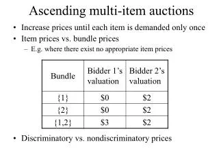
2. Multi-item auctions • Auctioning multiple distinguishable items when bidders have preferences over combinations of items: complementarity & substitutability • Example applications • Allocation of transportation tasks • Allocation of bandwidth • Dynamically in computer networks • Statically e.g. by FCC • Manufacturing procurement • Electricity markets • Securities markets • Liquidation • Reinsurance markets • Retail ecommerce: collectibles, flights-hotels-event tickets • Resource & task allocation in operating systems & mobile agent platforms

3. Mechanism design for multi-item auctions • Sequential auctions • How should rational agents bid (in equilibrium)? • Full vs. partial vs. no lookahead • Would need normative deliberation control methods • Inefficiencies can result from future uncertainties • Parallel auctions • Inefficiencies can still result from future uncertainties • Postponing & minimum participation requirements • Unclear what equilibrium strategies would be • Methods to tackle the inefficiencies • Backtracking via reauctioning (e.g. FCC [McAfee&McMillan96]) • Backtracking via leveled commitment contracts [Sandholm&Lesser95,AAAI-96, GEB-01] [Sandholm96] [Andersson&Sandholm98a,b] • Breach before allocation • Breach after allocation

4. Mechanism design for multi-item auctions... • Combinatorial auctions[Rassenti,Smith&Bulfin82]... • Bids can be submitted on combinations (bundles) of items • Bidder’s perspective • Avoids the need for lookahead • (Potentially 2#items valuation calculations) • Auctioneer’s perspective: • Automated optimal bundling of items • Winner determination problem: • Label bids as winning or losing so as to maximize sum of bid prices (= revenue  social welfare) • Each item can be allocated to at most one bid • Exhaustive enumeration is 2#bids

6. Level {2},{3},{1,4} {1},{2},{3,4} {3},{4},{1,2} {1},{3},{2,4} {1},{4},{2,3} {1},{2,3,4} {2},{4},{1,3} {1,3},{2,4} {3},{1,2,4} {1,4},{2,3} {4},{1,2,3} {1,2,3,4} {1,2},{3,4} {2},{1,3,4} {1}{2}{3}{4} (4) (3) (2) (1) Space of allocations #partitions is (#items#items/2), O(#items#items) [Sandholm et al. AAAI-98, AIJ-99, Sandholm AIJ-02] Another issue: auctioneer could keep items

7. 1 1,2 [Rothkopf et al. Mgmt Sci 98] 2 1,3 1,2,3 3 2,3 Dynamic programming for winner determination • Uses (2#items), O(3#items) operations independent of #bids • (Can trivially exclude items that are not in any bid) • Does not scale beyond 20-30 items

8. NP-completeness • NP-complete [Rothkopf et al Mgmt Sci 98] • Weighted set packing [Karp 72] • [For an overview of worst-case complexity results of the winner determination problem, see review article by Lehmann, Mueller, and Sandholm in the textbook Combinatorial Auctions, MIT Press 2006 • available at www.cs.cmu.edu/~sandholm]

9. Polynomial time approximation algorithms with worst case guarantees value of optimal allocation k = value of best allocation found General case • Cannot be approximated to k = #bids1-  (unless probabilistic polytime = NP) • Proven in [Sandholm IJCAI-99, AIJ-02] • Reduction from MAXCLIQUE, which is inapproximable [Håstad96] • Best known approximation gives k = O(#bids / (log #bids)2 ) [Haldorsson98]

10. Polynomial time approximation algorithms with worst case guarantees Special cases • Let  be the max #items in a bid: k= 2 / 3 [Haldorsson SODA-98] • Bid can overlap with at most  other bids: k= min( (+1) / 3 , (+2) / 3,  / 2 ) [Haldorsson&Lau97;Hochbaum83] • k= sqrt(#items) [Haldorsson99] • k= chromatic number / 2 [Hochbaum83] • k=[1 + maxHG minvH degree(v) ] / 2 [Hochbaum83] • Planar: k=2 [Hochbaum83] • So far from optimum that irrelevant for auctions • Probabilistic algorithms? • New special cases, e.g. based on prices [Lehmann et al. 01]

11. 1 2 6 |set|  2 3 5 or |set| > #items / c 4 1 2 3 4 5 6 7 O(n #items ) c-1 3 O(#items ) 2 large or NP-complete already O(#items ) 3 if 3 items per bid are allowed Restricting the allowable combinations that can be bid on to get polytime winner determination [Rothkopf et al. Mgmt Sci 98] Gives rise to the same economic inefficiencies that prevail in noncombinatorial auctions

12. [Sandholm & Suri AAAI-00, AIJ-03]

13. Item graphs[Conitzer, Derryberry, Sandholm AAAI-04] Caltrain ticket • Item graph = graph with the items as vertices where every bid is on a connected set of items • Example: Ticket to Children’s Museum, San Jose Ticket to Alcatraz, San Francisco Rental car Bus ticket • Does not make sense to bid on items in SF and SJ without transportation • Does not make sense to bid on two forms of transportation

14. Clearing with item graphs • Tree decomposition of a graph G = a tree T with • Subsets of G’s vertices as T’s vertices; for every G-vertex, set of T-vertices containing it must be a nonempty connected set in T • Every neighboring pair of vertices in G occurs in some single vertex of T • Width of T = (max #G-vertices in single T-vertex)-1 • (For bounded width, can construct tree decomposition of width w in polynomial time (if it exists)) • Thrm. Given an item graph with tree decomposition T (width w), can clear optimally in time O(|T|2 (|Bids|+1)w+1) • Sketch: for every partial assignment of a T-vertex’s items to bids, compute maximum possible value below that vertex (using DP)

15. t1 t2 t3 t4 resource 1 … invalid bid resource 2 resource 3 valid bid Application: combinatorial renting • There are multiple resources for rent • “item” = use of a resource for a particular time slot • Assume every bid demands items in a connected interval of time periods • Green edges give valid item graph • width O(#resources) • can also allow small time gaps in bids by drawing edges that skip small numbers of periods

16. s1 s2 s3 s4 resource 1 … resource 2 resource 3 Application: conditional awarding of items • Can also sell a type of security: you will receive the resource iff state si of the world materializes • simust be disjoint so that we never award resource twice • States potentially have a linear order • e.g. s1 = “price of oil < $40,” s2 = “$40 < price of oil < $50,” s3 = “$50 < price of oil < $60,” … • If each bid demands items in connected set of states, then technically same as renting setting

17. Generalization: substitutability [Sandholm IJCAI-99, AIJ-02] • What if agent 1 bids • $7 for {1,2} • $4 for {1} • $5 for {2} ? • Bids joined with XOR • Allows bidders to express general preferences • Groves-Clarke pricing mechanism can be applied to make truthful bidding a dominant strategy • Worst case: Need to bid on all 2#items-1 combinations • OR-of-XORs bids maintain full expressiveness & are more concise • E.g. (B2XOR B3) OR (B1XOR B3XOR B4) OR ... • Our algorithm applies (simply more edges in bid graph => faster) • Preprocessors do not apply • Short bid technique & interval bid technique do not apply • XOR-of-ORs [Nisan EC-00] • OR* [Nisan EC-00] = phantom items [Fujishima et al. IJCAI-99]

18. Side constraints in markets • Traditionally, markets (auctions, reverse auctions, exchanges) have been designed to optimize unconstrained economic value (revenue/cost/surplus) • Side constraints • Required in many practical markets to encode legal, contractual and business constraints • Could be imposed by any party • Sellers • Buyers • Auctioneer • Market maker • … • Can make fully expressive bidding exponentially more compact • Have significant implications on complexity of market clearing

19. Complexity implications of side constraints[Sandholm & Suri IJCAI-01 workshop on Distributed Constraint Reasoning] • Noncombinatorial multi-item auctions are solvable in polynomial time • Thrm. Budget constraints: NP-complete • Max number of items per bidder: polynomial time [Tennenholtz 00] • Thrm. Max winners: NP-complete even if bids can be accepted partially • Thrm. XORs: NP-complete & inapproximable even if bids can be accepted partially • These results hold whether or not seller has to sell all items • Combinatorial auctions are polynomial time if bids can be accepted partially • Some side constraint types (e.g. max winners, XORs) make problem NP-complete • Counting constraints • Other constraints allow polynomial time clearing • Cost constraints: mutual business, trading volume, minorities, … • Unit constraints, … • Some side constraints can make NP-hard combinatorial auction clearing easy ! • These results apply to exchanges & reverse auctions also

20. Tree search-based winner determination algorithms for combinatorial auctions and generalizations

21. Solving the winner determination problem when all combinations can be bid on:Search algorithms for optimal anytime winner determination • Capitalize on sparsely populated space of bids • Generate only populated parts of space of allocations • Highly optimized • 1st generation algorithm: branch-on-items formulation [Sandholm ICE-98, IJCAI-99, AIJ-02; Fujishima, Leyton-Brown & Shoham IJCAI-99] • 2nd generation algorithm: branch-on-bids formulation [Sandholm&Suri AAAI-00, AIJ-03, Sandholm et al. IJCAI-01] • New ideas, e.g., multivariate branching

22. Bids: 1 2 1 1,2 1,3,5 1,4 3 4 5 2 3 2 3,5 2,5 2,5 2 1,2 1,3,5 1,4 4 4 4 3 3,5 3 3 3,5 3 2,5 3,5 5 5 4 4 4 5 First generation search algorithms: branch-on-items formulation [Sandholm ICE-98, IJCAI-99, AIJ-02]

23. B A Bid graph A D C IN OUT B C B D C C OUT IN IN OUT C D C OUT IN D D IN OUT 2nd generation algorithm: Combinatorial Auction, Branch On Bids[Sandholm&Suri AAAI-00, AIJ-03] Bids of this example A={1,2} B={2,3} C={3} D={1,3} • Finds an optimal solution • Naïve analysis: 2#bids leaves • Thrm. At most leaves • where k is the minimum #items per bid • provably polynomial in bids even in worst case!

24. Use of h-values (=upper bounds) to prune winner determination search • f* = value of best solution found so far • g = sum of prices of bids that are IN on path • h = value of LP relaxation of remaining problem • Upper bounding: Prune the path when g+h ≤ f*

25. Linear programming for computing h-values

26. Linear program of the winner determination problem aka shadow price

27. Linear programming Original problem maximize such that Initial tableau Slack variables Assume, for simplicity, that origin is feasible (otherwise have to run a different LP to find first feasible and run the main LP in a revised space). Simplex method “pivots” variables in and out of the tableau Basic variables are on the left hand side

28. Graphical interpretation of simplex algorithm for linear programming Entering variable x1 x2 Departing variable Departing variable is slack variable of the constraint Constraints c Feasible region Each pivot results in a new tableau Entering variable x2 x1

29. Speeding up the use of linear programs in search • If LP returns a solution where all integer variables have integer values, then that is the solution to that node and no further search is needed below that node • Instead of simplex in the LP, use simplex in the DUAL because after branching, the previous DUAL solution is still feasible and a good starting point for simplex at the new node • Thrm. LP optimum value = DUAL optimum value aka shadow price

30. The branch-and-cut approach

31. Cutting planes (aka cuts) • Extra linear constraints can be added to the LP to reduce the LP polytope and thus give tighter bounds (less optimistic h-values) if the constraints are guaranteed to not exclude any integer solutions • Applications-specific vs. general-purpose cuts • Branch-and-cut algorithm = branch-and-bound algorithm that uses cuts • A global cut is valid throughout the search tree • A local cut is guaranteed to be valid only in the subtree below the node at which it was generated (and thus needs to be removed from consideration when not in that subtree)

32. Example of a cut that is valid for winner determination: Odd hole inequality E.g., 5-hole x8 x3 x2 No chord x1 x6 Edge means that bids share items, so both bids cannot be accepted x1 + x2 + x3 + x6 + x8 ≤ 2

33. Valid cut that separates Valid cut that does not separate Invalid cut Separation using cuts LP optimum

34. How to find cuts that separate? • For some cut families (and/or some problems), there are polynomial-time algorithms for finding a separating cut • Otherwise, use: • Generate a cut • Generation preferably biased towards cuts that are likely to separate • Test whether it separates

35. Gomory mixed integer cut • Powerful general-purpose cut • Applicable to all problems, where • constraints and objective are linear, • the problem has integer variables and potentially also real variables • Cut is generated using the LP optimum so that the cut separates Curiosity: the problem could be solved with no search by an algorithm that generates a finite (potentially exponential) number of these cuts. (This assumes integer variables; can be extended to incorporate continuous variables too, but finite convergence is no longer guaranteed.)

36. Integer variable (not a slack variable) LHS and RHS differ by an integer Derivation of Gomory mixed integer cut Input: optimal tableau row Define: non-basic, integer, continuous Rewrite tableau row: All integer terms add up to integers:

37. Back to search for winner determination…

38. Structural improvements to search algorithms for winner determinationOptimum reached faster & better anytime performance • Always branch on a bid j that maximizes e.g. pj / |Sj| (presort) • Lower bounding: If g+L>f*, then f*g+L • Identify decomposition of bid graph in O(|E|+|V|) time & exploit • Pruning across subproblems (upper & lower bounding) by using f* values of solved subproblems and h values of yet unsolved ones • Forcing decomposition by branching on an articulation bid • All articulation bids can be identified in O(|E|+|V|) time • Could try to identify combinations of bids that articulate (cutsets)

40. Question ordering heuristics • In depth-first branch-and-bound, it is best to branch on a question for which the algorithm knows a good answer with high likelihood • Best (to date) heuristics for branching on bids[Sandholm,Suri,Gilpin&Levine IJCAI-01]: • A: Branch on bid whose LP value is closest to 1 • B: Branch on bid with highest normalized shadow surplus: • Choosing the heuristic dynamically based on remaining subproblem • E.g. use A when LP table density > 0.25 and B otherwise • In A* search, it is best to branch on a question whose right answer the algorithm is very uncertain about • Early branch-and-bound algorithms branched on variable whose LP value is most fractional • More general idea [Gilpin&Sandholm 07]: branch on a question that reduces the entropy of the LP solution the most • Determine this e.g. based on lookahead • Applies to multivariate branching too

41. Identifying & solving tractable cases at search nodes(so that no search is needed below such nodes) [Sandholm & Suri AAAI-00, AIJ-03]

42. Example 1: “Short” bids [Sandholm&Suri AAAI-00, AIJ-03] • Never branch on short bids with 1 or 2 items • At each search node, we solve short bids from bid graph separately • O(#short bids 3) time using maximal weighted matching • [Edmonds 65; Rothkopf et al 98] • NP-complete even if only 3 items per bid allowed • Dynamically delete items included in only one bid

43. Example 2: Interval bids • At each search node, use a polynomial algorithm if remaining bid graph only contains interval bids • Ordered list of items: 1..#items • Each bid is for some interval [q, r] of these items • [Rothkopf et al. 98] presented O(#items2) DP algorithm • [Sandholm&Suri AAAI-00, AIJ-03] DP algorithm is O(#items + #bids) • Bucket sort bids in ascending order of r • opt(i) is the optimal solution using items 1..i • opt(i) = max b in bids whose last item is i {pb + opt(qb-1), opt(i-1)} • Identifying linear ordering • Can be identified in O(|E|+|V|) time [Korte & Mohring SIAM-89] • Interval bids with wraparound can be identified in O(#bids2) time [Spinrad SODA-93] and solved in O(#items (#items + #bids)) time using our DP while DP of Rothkopf et al. is O(#items3)

44. Example 3: [Sandholm & Suri AAAI-00, AIJ-03]

45. Example 3... • Thrm. [Conitzer, Derryberry & Sandholm AAAI-04]An item tree that matches the remaining bids (if one exists) can be constructed in time O(|Bids| |#items that any one bid contains|2 + |Items|2) • Algorithm: • Make a graph with the items as vertices • Each edge (i, j) gets weight #(bids with both i and j) • Construct maximum spanning tree of this graph: O(|Items|2) time • Thrm. The resulting tree will have the maximum possible weight #(occurrences of items in bids) - |Bids| iff it is a valid item tree • Complexity of constructing an item graph of treewidth k is NP-complete for k=3 or more [Gottlob & Greco EC-07] • But complexity of solving any such case given the item graph is “polynomial-time” - exponential only in the treewidth • Another polynomially solvable case that subsumes the structured item graph case is presented in [Gottlob & Greco EC-07]

46. Other generalizations of combinatorial auctions[Sanholm, Suri, Gilpin & Levine IJCAI-01 workshop, AAMAS-02] • Free disposal vs. no free disposal • Single vs. multiple units of each item • Auction vs. reverse auction vs. exchange • Reservation prices

47. Combinatorial reverse auction • Example: procurement in supply chains • Auctioneer wants to buy a set of items (has to get all) • Can take extras if there is free disposal • Sellers place bids on how cheaply they are willing to sell bundles of items • Thrm. Winner determination is NP-complete even in single-unit case with free disposal • Thrm. Single unit case with free disposal is approximable • k = 1 + log m (m = largest number of items that any bid contains) • Greedy algorithm: Keep choosing bid with lowest price / #items

48. No free disposal • Free disposal: seller can keep items, buyers can take extras • Free disposal usually assumed in the combinatorial auction literature • In practice, freeness of disposal can vary across items & bidders • Without free disposal, the set of feasible solutions is same for combinatorial auctions & reverse auctions • Thrm. Without free disposal, even finding a feasible solution is NP-complete

49. Combinatorial exchange • Example bid: (buy 20 tons of water, sell 10 cubic meters of hydrogen, sell 5 cubic meters of oxygen, ask $500) • Example application: manufacturing where a participant bids for inputs & outputs of a production plan simultaneously • Label bids as winning or losing so as to maximize (revealed) surplus: sum of amounts paid by bidders minus sum of amounts paid to bidders • On each item, sell quantity  buy quantity • Equality if there is no free disposal • Alternatively, could maximize liquidity (trading volume) • Thrm. NP-complete even in the single-unit case • Thrm. Inapproximable even in the single-unit case • Thrm. Without free disposal, even finding a feasible solution is NP-complete (even in the single-unit case)

50. What if some bids acceptable fractionally?[Kothari, Suri & Sandholm ACM-EC-03] • Q: How many bids have to be accepted fractionally (in worst case) so as to obtain maximum surplus in a multi-item multi-unit combinatorial exchange / combinatorial auction? • Trivial answer: #bids • A: #items (this is independent of #units) • Q: How many bids have to be accepted fractionally (in worst case) so as to maximize liquidity in a multi-item multi-unit combinatorial exchange? • Trivial answer: #bids • A: #items + 1 (this is independent of #units) • Q: How complex is it to find such a solution? • A: Can be found using any LP algorithm that terminates in an optimal vertex of the LP polytope