Download
1 / 33
380 likes | 909 Views
MAE 3130: Fluid Mechanics Lecture 4: Bernoulli Equation Spring 2003. Dr. Jason Roney Mechanical and Aerospace Engineering. Outline. Introduction Newton’s Second Law Along a Streamline Normal to a Streamline Physical Interpretation Static, Stagnation, Dynamic and Total Pressure

E N D
MAE 3130: Fluid MechanicsLecture 4: Bernoulli EquationSpring 2003 Dr. Jason Roney Mechanical and Aerospace Engineering
Outline • Introduction • Newton’s Second Law • Along a Streamline • Normal to a Streamline • Physical Interpretation • Static, Stagnation, Dynamic and Total Pressure • Use of the Bernoulli Equation • Examples
Bernoulli’s Equation: Introduction Swiss mathematician, son of Johann Bernoulli, who showed that as the velocity of a fluid increases, the pressure decreases, a statement known as the Bernoulli principle. He won the annual prize of the French Academy ten times for work on vibrating strings, ocean tides, and the kinetic theory of gases. For one of these victories, he was ejected from his jealous father's house, as his father had also submitted an entry for the prize. His kinetic theory proposed that the properties of a gas could be explained by the motions of its particles. Daniel Bernoulli (1700-1782) • Acceleration of Fluid Particles give Fluid Dynamics • Newton’s Second Law is the Governing Equation • Applied to an Idealized Flow and Assumes Inviscid Flow • There are numerous assumptions • “Most Used and Abused Equation” The Bernoulli Equation is Listed in Michael Guillen's book "Five Equations that Changed the World: The Power and Poetry of Mathematics"
Newton’s Second Law: Fluid Dynamics F are the forces acting on the fluid particle, m is the mass of a fluid particle, and a is the acceleration of the fluid particle Possible Forces: Body Forces and Surface Forces Surface Forces: Pressure and Shear Stresses Body Forces: Gravity, Magnetic Fields, etc. Consider Inviscid Flow: If a flow is inviscid, it has zero viscosity, and likewise no thermal conductivity or heat transfer. In practice, there are no inviscid fluids, since all fluids support shear. In some flows, the viscous effect is very small, confined to a thin layer. Water flows can be of either type, a lot of gases have situation where viscosity is negligible
Newton’s Second Law: Fluid Dynamics Thus, for this lecture, we only consider Pressure and Gravity Forces using the inviscid approximation: This balance of forces on fluid has numerous applications in Fluid Dynamics All fluid flows contain three dimensions and time. Cartesian Coordinates, (x, y, z) and Cylindrical Coordinates, (r, q, z) are common coordinates used in fluid dynamics. For this lecture we will concern ourselves with flows in the x-z plane.
Newton’s Second Law: Fluid Dynamics We describe the motion of each particle with a velocity vector: V Particles follow specific paths base on the velocity of the particle. Location of particle is based on its initial position at an initial time, and its velocity along the path. If the flow is a steady flow, each successive particle will follow the same path.
Newton’s Second Law: Steady Flow For Steady Flow, each particle slides along its path, and the velocity vector is every tangent to the path. The lines that the velocity vectors are tangent to are called streamlines. We can introduce streamline coordinate, s(t) along the streamline and n, normal to the streamline. Then (s) is the radius of curvature of the streamline.
Newton’s Second Law: Steady Flow For 2-D Flows, there are two acceleration components: s-direction by chain rule: Normal direction (n) is the centrifugal acceleration: In general there is acceleration along the streamline: There is also acceleration normal to the streamline: However, to produce an acceleration there must be a force!
Newton’s Second Law: Steady Flow F.B.D. Remove, the fluid particle from its surroundings. Draw the F.B.D. of the flow. Assume pressure forces and gravity forces are important. Neglect surface tension and viscous forces.
Newton’s Second Law: Along a Streamline Use Streamline coordinates, our element is ds x dn x dy, and the unit vectors are n and s, and apply Newton’s Second Law in the Streamline Direction. Streamline, F = ma: Gravity Forces: Pressure Forces (Taylor Series): arises since pressures vary in a fluid P is the pressure at the center of the element Shear Forces: Neglected, Inviscid!
Newton’s Second Law: Along a Streamline Then, = Divide out volume, recall The change of fluid particle speed is accomplished by the appropriate combination of pressure gradient and particle weight along the streamline. In a static fluid the R.H.S is zero, and pressure and gravity balance. In a dynamic fluid, the pressure and gravity are unbalanced causing fluid flow.
Newton’s Second Law: Along a Streamline Note, we can rewrite terms in the above equation: 0 = constant along a streamline Then, Simplify,
Newton’s Second Law: Along a Streamline Integrate, In general, we can not integrate the pressure term because density can vary with temperature and pressure; however, for now we assume constant density. Then, Celebrated Bernoulli’s Equation Assumptions: Balancing Ball: • Viscous effects are assumed negligible (inviscid). • The flow is assumed steady. • The flow is assume incompressible. • The equation is applicable along a streamline. * We can apply along a streamline in planar and non-planar flows!
Newton’s Second Law: Normal to a Streamline Normal, F = ma: Gravity Forces: Pressure Forces (Taylor Series): arises since pressures vary in a fluid P is the pressure at the center of the element Shear Forces: Neglected, Inviscid!
Newton’s Second Law: Normal to a Streamline Then, Divide out volume, recall A change in direction of a flow of a fluid particle speed is accomplished by the appropriate combination of pressure gradient and particle weight normal to the streamline. A large force unbalance is needed for motion resulting from a large V or r or small . In gravity is neglected (gas flow): Pressure increases with distance away from the center of curvature, as in a tornado or Hurricane where at the then center the low pressure creates vacuum conditions.
Newton’s Second Law: Normal to a Streamline Hurricane Pick a Streamline 1013 mb 922 mb at Eye Now, using the hydrostatic condition, how high would the sea level rise due to lower pressure ? Free Vortex:
Newton’s Second Law: Normal to a Streamline Multiply the above equation by dn, and assume that s is constant, such that, Integrate, Assume density is constant, incompressible, however, we do not know Thus, for across streamlines for steady, incompressible, inviscid flow:
Physical Interpretation: Normal and Along a Streamline • Basic Assumptions: • Steady • Inviscid • Incompressible • A violation of one or more of the assumptions mean the equation is invalid. • The “Real World” is never entirely all of the above. • If the flow is nearly Steady, Incompressible, and Inviscid, it is possible to adequately model it. The three terms that the equations model are: pressure, acceleration, and weight. Acceleration Weight Pressure The Bernoulli equation is a statement of the work-energy principle: The work done on a particle by all forces acting on the particle is equal to the change of kinetic energy of the particle.
Physical Interpretation: Normal and Along a Streamline As a fluid particle moves, pressure and gravity both do work on the particle: p is the pressure work term, and gz is the work done by weight. 1/2rV2 is the kinetic energy of the particle. Alternatively, the Bernoulli equation can be derived from the first and second laws of Thermodynamics (energy and entropy) instead of the Newton’s 2nd Law with the appropriate restrictions. Bernoulli’s Equation can be written in terms of heads: Pressure Head Elevation Term Velocity Head Pressure Head: represents the height of a column of fluid that is needed to produce the pressure p. Velocity Head: represents the vertical distance needed for the fluid to fall freely to reach V. Elevation Term: related to the potential energy of the particle.
Physical Interpretation: Normal and Along a Streamline • For Steady Flow the acceleration can be interpreted as arising from two distinct sources: • Change in speed along a streamline • Change in direction along a streamline Bernoulli Equation gives (1), change in Kinetic Energy. Integration Normal to the Streamline gives (2), Centrifugal Acceleration. In many cases , and the centrifugal effects are negligible, meaning the pressure variation is hydrostatic even though the fluid is in motion.
Static, Stagnation, Dynamic, and Total Pressure: Bernoulli Equation Hydrostatic Pressure Dynamic Pressure Static Pressure Static Pressure: moves along the fluid “static” to the motion. Dynamic Pressure: due to the mean flow going to forced stagnation. Hydrostatic Pressure: potential energy due to elevation changes. Following a streamline: Follow a Streamline from point 1 to 2 0 0, no elevation 0, no elevation “Total Pressure = Dynamic Pressure + Static Pressure” Note: H > h In this way we obtain a measurement of the centerline flow with piezometer tube.
Stagnation Point: Bernoulli Equation Stagnation point: the point on a stationary body in every flow where V= 0 Stagnation Streamline: The streamline that terminates at the stagnation point. Symmetric: Stagnation Flow I: Axisymmetric: If there are no elevation effects, the stagnation pressure is largest pressure obtainable along a streamline: all kinetic energy goes into a pressure rise: Stagnation Flow II: Total Pressure with Elevation:
Pitot-Static Tube: Speed of Flow p2 = p3 p2 p1 p1 = p4 H. De Pitot (1675-1771) p1 p2 p1 p2 p1 p2 Stagnation Pressure occurs at tip of the Pitot-static tube: Static Pressure occurs along the static ports on the side of the tube: (if the elevation differences are negligible, i.e. air) Now, substitute static pressure in the stagnation pressure equation: Air Speed: Now solve for V:
Pitot-Static Tube: Design • Pitot-static probes are relatively simple and inexpensive • Depends on the ability to measure static and stagnation pressure • The pressure values must be obtained very accurately Sources of Error in Design in the Static Port: A) Burs Sources of Error in Design in the Static Port: C) Alignment in Flow Yaw Angle of 12 to 20 result in less than 1% error. OK Error: Accelerates Error: Stagnates Sources of Error in Design in the Static Port: B) Spacing Too Close
Pitot-Static Tube: Direction of Flow A Pitot-static Probe to determine direction: v Rotation of the cylinder until p1 and p3 are the same indicating the hole in the center is pointing directly upstream. P2 is the stagnation pressure and p1 and p3 measure the static pressure. b is at the angle to p1 and p3 and is at 29.5. The equation with this type of pitot-static probe is the follwing:
Uses of Bernoulli Equation: Free Jets New form for along a streamline between any two points: If we know 5 of the 6 variable we can solve for the last one. Free Jets: Case 1 Torricelli’s Equation (1643): Note: p2 = p4 by normal to the streamline since the streamlines are straight. Following the streamline between (1) and (2): As the jet falls: 0 0 h 0 gage 0 gage V
Uses of Bernoulli Equation: Free Jets Free Jets: Case 2 =g(h-l) 0 0 l 0 gage V Then, Physical Interpretation: All the particles potential energy is converted to kinetic energy assuming no viscous dissipation. The potential head is converted to the velocity head.
Uses of Bernoulli Equation: Free Jets Free Jets: Case 3 “Horizontal Nozzle: Smooth Corners” However, we calculate the average velocity at h, if h >> d: Slight Variation in Velocity due to Pressure Across Outlet Torricelli Flow: Free Jets: Case 4 “Horizontal Nozzle: Sharp-Edge Corners” vena contracta: The diameter of the jet dj is less than that of the hole dh due to the inability of the fluid to turn the 90° corner. The pressure at (1) and (3) is zero, and the pressure varies across the hole since the streamlines are curved. The pressure at the center of the outlet is the greatest. However, in the jet the pressure at a-a is uniform, we can us Torrecelli’s equation if dj << h.
Uses of Bernoulli Equation: Free Jets Free Jets: Case 4 “Horizontal Nozzle: Sharp-Edge Corners” Vena-Contracta Effect and Coefficients for Geometries
Uses of the Bernoulli Equation: Confined Flows There are some flow where we can-not know the pressure a-priori because the system is confined, i.e. inside pipes and nozzles with changing diameters. In order to address these flows, we consider both conservation of mass (continuity equation) and Bernoulli’s equation. Consider flow in and out of a Tank: The mass flow rate in must equal the mass flow rate out for a steady state flow: and With constant density,
Uses of the Bernoulli Equation: Final Comments In general, an increase in velocity results in a decrease in pressure. Flow in a Pipe: Airplane Wings: Venturi Flow:
Uses of Bernoulli Equation: Flow Rate Measurement Flowrate Measurements in Pipes using Restriction: Horizontal Flow: An increase in velocity results in a decrease in pressure. Assuming conservation of mass: Substituting we obtain: So, if we measure the pressure difference between (1) and (2) we have the flow rate.


![BIO 208 FLUID FLOW OPERATIONS IN BIOPROCESSING [ 3 1 0 4 ]](https://cdn3.slideserve.com/5612051/bio-208-fluid-flow-operations-in-bioprocessing-3-1-0-4-dt.jpg)