Download
1 / 17
170 likes | 375 Views
Time-series modelling of aggregate wind power output. Alexander Sturt, Goran Strbac 17 March 2011. Introduction. Eastern Wind Integration and Transmission Study (EWITS) (2010). Wind datasets prepared by AWS Truewind over 9 month period

E N D
Time-series modelling of aggregate wind power output Alexander Sturt, Goran Strbac 17 March 2011
Introduction Eastern Wind Integration and Transmission Study (EWITS) (2010) • Wind datasets prepared by AWS Truewind over 9 month period • Created by simulation using mesoscale Numerical Weather Prediction (NWP) model • 3 years of synthetic data, 1326 sites (freely available online) • Hardware used: 80 x dual CPU quad core penguin workstations (640 cores) • Run time per year of simulation: 21 days (in theory...) What if this level of detail isn’t needed? What if we need a model of aggregated wind output? What if we need to understand the statistical properties?
Modelling strategy • Univariate model for aggregate wind power, not wind speed • Autoregressive driver: AR(p), hourly (or half-hourly) timesteps • Include diurnal variation with periodic additive term: • Fit to long-term distribution with transformation function: • Use different models for the different seasons iid N(0,1) n = number of data points per day
Model calibration 1. Choose these to satisfy long-term distribution and diurnal variation, assuming X~N(0,1) X P W Σ μ
Model calibration 2. Choose parameters of AR model to fit short-term transitional properties and N(0,1) asymptotic distribution X P W Σ μ
Case study: GB2030 model • 6 years of hourly wind speed data taken from MIDAS dataset by Olmos (2009) • 116 sites (onshore only) • 10m anemometer data extrapolated to hub-height and converted to wind power using turbine curve • Regional weightings chosen to match core 2030 buildout scenario used by Poyry (2009); offshore capacity mapped to nearest onshore regions Olmos Poyry
GB2030: modelling strategy • Weighted regional power output aggregated to produce a univariate time series • Split into four seasons • For each season, calibrate model to reproduce asymptotic distribution, diurnal variation and short-term volatility, using AR(2) model • Tweak to approximate effect of offshore component
GB2030 (untweaked): distribution and volatility Volatility curve Power output distribution
GB2030 (untweaked):distribution of absolute power output changes 1 hr 4 hr 8 hr 24 hr
What about turbine cutout? Denmark, distribution of 4-hour changes (non-rolling window) 8 Jan 2005
GB2030: tweaking strategy (1) • Diurnal variation is too great • Lunchtime wind speed peak at hub height is less pronounced than at anemometer height (insolation reduces stability) • Offshore component has no diurnality => Reduce μ values by a factor of 4
GB2030: tweaking strategy (2) • Offshore component increases mean capacity factor (28% -> 33%) • => Stretch W function so as to match duration curves shown in Poyry (2009). Use same AR parameters as untweaked model Synthetic data from tweaked GB2030 model Poyry 2030 data (43GW capacity)
GB2030: Effect of tweak Volatility curve Power output distribution
GB2030: Time history sample (“Turing test”) Wind output (GW) Poyry data Tweaked GB2030 synthetic winter data
Conclusions • Non-Gaussian wind power time series can be transformed to a Gaussian (X) domain and modelled with a Gaussian time series model • Synthetic time series reproduce the important long-term and transitional properties (for power system simulation) • Simplicity of model makes it possible to write down formulae for any desired statistic • Transformation to Gaussian domain simplifies modelling of correlated RVs: • Forecast errors (anti-correlated with wind realisation to prevent forecast biasing) • Multi-bus models • Combined demand / wind model
References • Sturt, A. and Strbac, G. “Time series modelling of power output for large-scale wind fleets”, Wind Energy, 2011 (to be published) • Enernex Corporation “Eastern Wind Integration and Transmission Study”, 2010 http://www.nrel.gov/wind/systemsintegration/ewits.html • Olmos, P. “Probability distribution of wind power during peak demand”, MSc dissertation, University of Edinburgh, 2009 • Olmos, P.E., Dent, C., Harrison, G.P. and Bialek, J.W. “Realistic calculation of wind generation capacity credits”, CIGRE/IEEE Symposium on integration of wide-scale renewable resources into the power delivery system, Calgary, 2009 • Poyry Energy Consulting, “Impact of intermittency: how wind variability could change the shape of the British and Irish electricity markets: summary report”, 2009 http://www.poyry.com • Sturt, A. and Strbac, G. “A time series model for the aggregate GB wind output circa 2030”, 2011http://www.ee.ic.ac.uk/%20alexander.sturt07/GB2030SOM.pdf