Download
1 / 39
500 likes | 1.23k Views
Lec 22 : Diesel cycle, Brayton cycle. For next time: Read: § 8-8 to 8-10. Methods section due Monday, November 17, 2003 Outline: Diesel cycle Brayton cycle Example problem Important points: Understand differences between the Otto, Diesel and Brayton cycles

E N D
For next time: • Read: § 8-8 to 8-10. • Methods section due Monday, November 17, 2003 • Outline: • Diesel cycle • Brayton cycle • Example problem • Important points: • Understand differences between the Otto, Diesel and Brayton cycles • Know how to compute the cycles using variable or constant specific heats • Know what components make up each of the cycles.
Brayton Cycle Proposed by George Brayton in 1870! http://www.pwc.ca/en_markets/demonstration.html
Other applications of Brayton cycle • Power generation - use gas turbines to generate electricity…very efficient • Marine applications in large ships • Automobile racing - late 1960s Indy 500 STP sponsored cars
TEAMPLAY • What expression of the first law applies? Why?
Brayton Cycle • 1 to 2--isentropic compression • 2 to 3--constant pressure heat addition (replaces combustion process) • 3 to 4--isentropic expansion in the turbine • 4 to 1--constant pressure heat rejection to return air to original state
Brayton Cycle • Because the Brayton cycle operates between two constant pressure lines, or isobars, the pressure ratio is important. • The pressure ratio is not a compression ratio.
Brayton cycle analysis As with any cycle, we’re going to concern ourselves with the efficiency and net work output: Efficiency: Net work:
Brayton cycle analysis 1 to 2 (isentropic compression in compressor), apply first law: When analyzing the cycle, we know that the compressor work is in (negative). It is standard convention to just drop the negative sign and deal with it later:
Brayton cycle analysis 2 to 3 (constant pressure heat addition - treated as a heat exchanger)
Brayton cycle analysis 3 to 4 (isentropic expansion in turbine)
Brayton cycle analysis 4 to 1 (constant pressure heat rejection) We know this is heat transfer out of the system and therefore negative. In book, they’ll give it a positive sign and then subtract it when necessary.
Brayton cycle analysis Let’s get the net work: Substituting:
Brayton cycle analysis Let’s get the efficiency:
Brayton cycle analysis Let’s assume cold air conditions and manipulate the efficiency expression:
Brayton cycle analysis Using the isentropic relationships, Let’s define:
Brayton cycle analysis Then we can relate the temperature ratios to the pressure ratio: Plug back into the efficiency expression and simplify:
Brayton cycle analysis An important quantity for Brayton cycles is the Back Work Ratio (BWR). Why might this be important?
The Back-Work Ratio is the Fraction of Turbine Work Used to Drive the Compressor
EXAMPLE PROBLEM • The pressure ratio of an air standard Brayton cycle is 4.5 and the inlet conditions to the compressor are 100 kPa and 27C. The turbine is limited to a temperature of 827C and mass flow is 5 kg/s. Determine • a) the thermal efficiency • b) the net power output in kW • c) the BWR • Assume constant specific heats.
Start analysis Let’s get the efficiency: From problem statement, we know rp = 4.5
Net power output: Net Power: Substituting for work terms: Applying constant specific heats:
Need to get T2 and T4 Use isentropic relationships: T1 and T3 are known along with the pressure ratios:
Solving for temperatures: T2: T4: Net power is then:
Back Work Ratio Applying constant specific heats:
Brayton Cycle We can also do the analysis with variable specific heats….we’ll use relative pressures.
TEAMPLAY Work the same problem with EES using variable specific heats. How do the numbers change?
Brayton Cycle • In theory, as the pressure ratio goes up, the efficiency rises. The limiting factor is frequently the turbine inlet temperature. • The turbine inlet temp is restricted to about 1,700 K or 2,600 F. • Consider a fixed turbine inlet temp., T3
For fixed values of Tmin and Tmax, the net work of the Brayton cycle first increases with the pressure ratio, then reaches a maximum at rp=(Tmax/Tmin)k/[2(k-1)], and finally decreases
Brayton Cycle • Irreversibilities • We had wc = h2 – h1 for the ideal cycle, which was isentropic • And we had wt = h3 – h4 for the ideal isentropic cycle
Brayton Cycle • In order to deal with irreversibilities, we need to write the values of h2 and h4 as h2,s and h4,s. • Then
TEAMPLAY Problem 8-69


![Tricarboxylic acid cycle (TCA Cycle) [Kreb’s cycle] [Citric acid cycle]](https://cdn2.slideserve.com/5062555/tricarboxylic-acid-cycle-tca-cycle-kreb-s-cycle-citric-acid-cycle-dt.jpg)