Download
1 / 22
230 likes | 419 Views
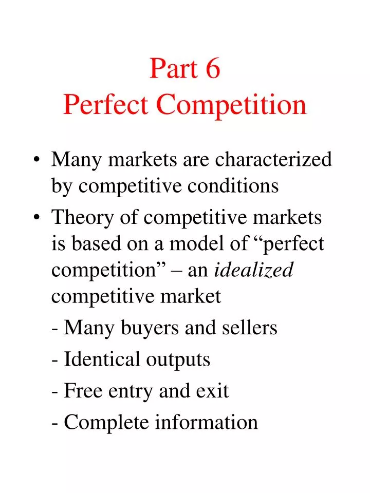
Part 6 Perfect Competition. Many markets are characterized by competitive conditions Theory of competitive markets is based on a model of “perfect competition” – an idealized competitive market - Many buyers and sellers - Identical outputs - Free entry and exit - Complete information.

E N D
Part 6Perfect Competition • Many markets are characterized by competitive conditions • Theory of competitive markets is based on a model of “perfect competition” – an idealized competitive market - Many buyers and sellers - Identical outputs - Free entry and exit - Complete information
The Firm Under Perfect Competition • Firm must be small relative to the size of the market (minimum efficient scale must be small relative to the market) • Individual firms cannot affect the market price (price taker) • Price is set in the market as a whole, the individual firm adjusts output so as to maximize profit given the market price
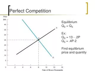
The Firm’s Total Revenue and Marginal Revenue Curves • As the market price is given, the firm’s total revenue is its output times the market price (P x Q) • The TR function will be a straight line from the origin • The firm’s marginal revenue is MR = ΔTR/ΔQ As all units of output sell for the same price MR = P
The Firm’s TR and MR Curves TR TR P = $1.25 125 Q 100 MR MR = P 1.25 Q
Profit Maximization • The firm has to decide whether to produce at all, and if so what output to produce • The firm will produce in the short run so long as its variable costs can be covered • Assuming the firm produces at all, the profit maximizing output is where there is the maximum excess of TR over TC or where MR = MC
Profit Maximum: TR and TC TC $ TR Economic Profit Q Q’ Q” Profit Max Profit 0 Q Q’ Q* Q” Loss Profit/Loss
Profit Maximum: MR and MC $ MC P MR Q Q* Why does MC = MR imply profit max? What would happen to TR and TC if output went up or down by a unit?
Profit in the Short Run MC $ MR P ATC Economic profit Q Q* $ MC Normal profit or break even ATC P MR Q Q*
Economic Loss in the Short Run $ MC ATC MR P Q* Q Economic loss Firm will produce Q* as long as P>AVC
Firm’s Short Run Supply Curve • The firm’s short run supply curve will be its MC curve above its AVC curve • If P is equal to or grater than Min AVC the firm will produce where P = MR = MC • If P < Min AVC the firm’s loss minimizing strategy is to shut down. Loss will equal TFC
Firm’s Short Run Supply Curve Break even or normal profit point $ ATC MC MR” P” P’ MR’ P MR Shut down point AVC Q Q” Q Q’ At prices below P the firm will shut down At prices between P and P’ the firm will produce where MC=MR at an economic loss At prices above P’ the firm will produce where MC=MR at an economic profit
Market Supply Curve • We can now derive the market supply curve • The supply curve of each firm is its MC curve above its min AVC point • The market supply curve is the horizontal sum of the supply curves of all the firms in the industry
Short Run Equilibrium of the Market and Firm • Market demand curve is the horizontal sum of all the demand curves of individuals • Short run market supply curve is the horizontal sum of all the short run supply curves of all the firms currently in the industry • Market price and quantity is determined by D = S • Each individual firm will produce at its profit max point of MR = MC
SR Equilibrium of Market and Firm Market equilibrium P S = ΣhMC P* D = ΣhDi Q Q* Equilibrium of the firm P MC MR P* ATC q q*
Shifts in Demand in the Short Run • Shifts in demand will create a movement along the market short run supply curve, changing market price • Each individual firm will adjust output to its new profit max level as price changes, moving along its own short run supply curve
Long Run Adjustments • In the long run capital is not fixed • Firms can change the size of their plants and move along their LAC curves • Firms can enter or leave the industry. They will enter if there is economic profit and leave if they are suffering economic losses • If firms change size or the number of firms in the industry changes the short run industry supply curve will shift • What conditions must hold for a perfectly competitive industry to be in long run equilibrium?
Long Run Equilibrium • Market price must adjust (via shifts in the short run supply curve) until all firms are just making normal profit • With normal profit there is no economic profit to attract new entrants and no economic losses to create exit • Also, for their to be no prospect of economic profit, price must equal minimum LAC • Otherwise firms could make economic profit by changing their plant size which would shift the SR supply curve of the industry
Long Run Equilibrium for Market and Firm P S = ΣhSMC P* D = ΣhDi Q Q* ATC SMC LAC MR P* q*
Long Run Supply Curve P S S’ P’ LRS P D’ D Q Q Q’ D shifts to D’, raising market price to P’. This will create excess profit for firms attracting new entrants and shifting S to S’ where all economic profit is again eliminated and new entry stops . This diagram shows a constant cost industry. Long run supply curve is horizontal
Possible Long Run Supply Curves • Constant cost industry -- horizontal LRS. Changes in the size of the industry do not affect firms’ costs of production • Increasing cost industry – upward sloping LRS. As an industry grows a factor price rises as a result, increasing costs for all firms • Decreasing cost industry – downward sloping LRS. As an industry grows a factor price falls as a result, decreasing costs for all firms—network effects • Technological change shifts the LRS
Are Competitive Markets Efficient? • In long run competitive equilibrium price is such that D=S and production is at min LAC • Productive efficiency—min LAC • The market D curve is can be interpreted as willingness to pay or marginal benefit curve • The market supply curve can be seen as the marginal opportunity cost of production curve • Competitive equilibrium is allocatively efficient (maximizes social surplus) provided all costs and benefits are reflected in the market D and S curves
Economic Inefficiencies • The efficient allocation may not be achieved even in competitive markets • Not all resources may be privately owned (open access resources) • It may not be possible for firms to capture peoples’ willingness to pay (public goods, external benefits) • Not all social costs may be reflected in the prices firms pay for factors of production (external costs) • Economic inefficiencies may also arise from lack of competition --Monopoly