Download
1 / 66
680 likes | 1.31k Views
Data Deluge in Times Series Analysis ("I need 1,000+ forecasts by end of day!"). Overview. Mass Forecasting vs. Data Mining Good ol’ fashioned forecasting ARIMA(X), ESMs , UCMs Data deluge (real world challenges) Building a good mass forecasting system 1 st attempts “The kitchen sink”

E N D
Data Deluge in Times Series Analysis("I need 1,000+ forecasts by end of day!")
Overview • Mass Forecasting vs. Data Mining • Good ol’ fashioned forecasting • ARIMA(X), ESMs, UCMs • Data deluge (real world challenges) • Building a good mass forecasting system • 1st attempts • “The kitchen sink” • Intelligent automation
Predictive Modeling (Data Mining) vs. Forecasting Predictive Modeling
Predictive Modeling (Data Mining) vs. Forecasting Forecasting
Predictive Modeling (Data Mining) vs. Forecasting Accuracy Profit AROC (c-sat) KS RMSE, SBC, AIC SE, SP GAIN LIFT Etc….
Predictive Modeling (Data Mining) vs. Forecasting TIME RMSE MAE MPE MAPE APE WAPE SBC, BIC R2 Random Walk R2 …and on and on and on…
Overview • Mass Forecasting vs. Data Mining • Good ol’ fashioned forecasting • ARIMA(X), ESMs, UCMs • Data deluge (real world challenges) • Building a good mass forecasting system • 1st attempts • “The kitchen sink” • Intelligent automation
The Universal Univariate Time Series Model TREND ERROR (Irregular) SEASONAL TRANSFORMATION
Additive Decomposition of the Airline Data T: Linear Trend S: Seasonal Average I: Irregular Component
Some SAS/ETS Procedures • ARIMA • AutoRegressive Integrated Moving Average models • Dynamic regression models (transfer function models) • AUTOREG • Simple regression models with autoregressive errors • ARCH and GARCH models (not covered) • FORECAST – ESM and autoregression models • UCM – Unobserved components models • SPECTRA – Spectral analysis • MODEL – Nonlinear modeling
Simple Exponential Smoothing Weights Y3 Y5 Y6 Y7 Y8 Y1 Y3 Y4 Y5 Y6 Y7 Y8 Y4 Y2 Weights applied to past values to predict Y9 The larger the parameter, the more the most recent values are emphasized. ...
ESM Models ESM Parameters Simple Double Linear (Holt) , Damped-Trend , , Seasonal , Additive Winters , , Multiplicative Winters , ,
Unobserved Components Models (UCMs) • Also known as structural time series models • Decompose time series into four components: • trend • season • cycle • irregular • General form: • Yt = Trend + Season + Cycle + Regressors
UCMs • Each component captures some important feature of the series dynamics. • Components in the model have their own models. • Each component has its own source of error. • The coefficients for trend, season, and cycle are dynamic. • The coefficients are testable. • Each component has its own forecasts.
UCM Procedure PROC UCM DATA=SAS-data-set ; ID variable INTERVAL=interval ; MODEL variable <=variables> ; IRREGULAR <options> ; LEVEL <options> ; SLOPE <options> ; SEASONLENGTH=n TYPE=DUMMY|TRIG <options> ; CYCLE <options> ; ESTIMATE OUTEST=SAS-data-set <options> ; FORECAST OUTFOR=SAS-data-set LEAD=n <options> ; RUN;
Box-Jenkins ARIMAX Models • ARIMAX: AutoRegressive Integrated Moving Average with eXogenous variables • AR: Autoregressive Time series is a function of its own past. • MA: Moving Average Time series is a function of past shocks (deviations, innovations, errors, and so on). • I: Integrated Differencing provides stochastic trend and seasonal components, so forecasting requires integration (undifferencing). • X: Exogenous Time series is influenced by external factors. (These input variables can actually be endogenous or exogenous.)
Autoregressive Moving Average Models A time series that is a linear function of p past values plus a linear combination of q past errors is called anautoregressive moving average process of order (p,q), denoted ARMA(p,q).
Additive Decomposition of the Airline Data T: Linear Trend S: Seasonal Average I: Irregular Component
Diagnosing Trend Year
Y t Y t Deterministic trends: Add function of time Linear Trend Quadratic Trend
Stochastic Trends: Use differencing Random walk with drift 1st Differenced RWD Take a simple difference
Seasonality? • SYt=Yt Yt-S , called a difference of order S. • Add seasonal dummy variables
ARIMA Procedure PROC ARIMA DATA=SAS-data-set ; BY variables ; IDENTIFY VAR=variable CROSS=(variables) NLAGS=n <options> ; ESTIMATE P=n Q=n INPUT=(variables) METHOD=CLS|ML|ULS <options> ; FORECAST OUT=SAS-data-set ID=variable INTERVAL=interval LEAD=n <options> ; RUN; QUIT;
Overview • Mass Forecasting vs. Data Mining • Good ol’ fashioned forecasting • ARIMA(X), ESMs, UCMs • Data deluge (real world challenges) • Building a good mass forecasting system • 1st attempts • “The kitchen sink” • Intelligent automation
Large-Scale Forecasting • Modern businesses require efficient, reliable forecasts for many series. These forecasts usually need to be updated on a regular basis. • There are too many series to manually implement the textbook approach for each one. • The series might be hierarchically arranged and require reconciliation of forecasts at different levels.
Forecasting a Large Number of Time Series • Compared to the single time series forecasting problem, when there are many time series to be forecast, the following conditions might occur: • There are not enough skilled analysts to provide forecasts for each series using conventional techniques. • Frequent forecast updates are usually required. • Time-stamped data must be converted to time-series data and managed automatically. • Exogenous variables or calendar events might influence the time series and must be included in automatic model selection.
Large-Scale Forecasting Scenario 80% can be forecast automatically. 10% requires extra effort. 10% cannot be forecast accurately. Time Series Data
Overview • Mass Forecasting vs. Data Mining • Good ol’ fashioned forecasting • ARIMA(X), ESMs, UCMs • Data deluge (real world challenges) • Building a good mass forecasting system • 1st attempts • “The kitchen sink” • Intelligent automation
A Good Mass Forecasting System • Requirements • Prepare Time Series Data • Fit many models • Allow for ‘sophisticated’ user defined models • Provide a variety of fit measures • Allow for hold-out assessment • Automatically pick ‘best’ models • Auto-diagnose data • Automatically incorporate events and inputs • Accommodate and reconcile hierarchies
Data Preparation:Equally Spaced Time Series Equally spaced time series Equally spaced time serieswith missing values Unequally spaced time series
Accumulate, Aggregate & Reconcile Accumulate Data Statistical Forecast Reconciled Forecast Daily Monthly Aggregate Data Reconcile Forecasts
TIMESERIES Procedure PROC TIMESERIES DATA=SAS-data-set OUT=SAS-data-set OUTDECOMP=SAS-data-set OUTSEASON=SAS-data-set OUTTREND=SAS-data-set SEASONALITY=n PRINT=(<options>) ; BY variables ; VAR variables ; DECOMP <TC><SC><IC><components> / MODE=ADD|MULT|mode ; ID variable INTERVAL=interval ; RUN;
FORECAST Procedure PROC FORECAST DATA=SAS-data-set OUT=SAS-data-set OUTEST=SAS-data-set TREND=1|2|3 METHOD=STEPAR|method-name AR=n SLENTRY=value SLSTAY=value INTERVAL=interval LEAD=n <options>; BY variables ; ID variables ; VAR variables ; RUN;
Summary of Data Used for Forecast Model Building Fit Sample Holdout Sample • Used to estimate model parameters for accuracy evaluation • Used to forecast values in holdout sample • Used to evaluate model accuracy • Simulates retrospective study Full = Fit + Holdout data is used to fit deployment model
Overview • Mass Forecasting vs. Data Mining • Good ol’ fashioned forecasting • ARIMA(X), ESMs, UCMs • Data deluge (real world challenges) • Building a good mass forecasting system • 1st attempts • “The kitchen sink” • Intelligent automation
Box-Jenkins Model Components Theoretical ARIMAX Model
The backshift operator Bk shifts a time series by k time units. Shift 1 time unit Shift 2 time units Shift k time units Backshift operator notation is a convenient way to write ARMA models. The Backshift Operator
Additive Decomposition of the Airline Data T: Linear Trend S: Seasonal Average I: Irregular Component
Model: Null Hypothesis: Alternative Hypothesis: The Dickey-Fuller Single Mean Test
The Dickey-Fuller Test in PROC ARIMA Augmented Dickey-Fuller Unit Root Tests Type Lags Rho Pr < Rho Tau Pr < Tau F Pr > F Zero Mean 0 -0.0214 0.6739 -0.12 0.6395 1 -0.0669 0.6636 -0.41 0.5309 2 -0.0265 0.6726 -0.22 0.6026 3 -0.0316 0.6713 -0.31 0.5682 4 -0.0152 0.6749 -0.18 0.6174 5 0.0005 0.6783 0.01 0.6803 Single Mean 0 -25.0564 0.0012 -4.01 0.0027 8.03 0.0010 1 -41.5691 0.0004 -4.97 0.0002 12.43 0.0010 2 -34.8515 0.0004 -3.66 0.0075 6.73 0.0073 3 -50.5816 0.0004 -3.75 0.0059 7.09 0.0010 4 -53.8412 0.0004 -3.20 0.0260 5.13 0.0428 5 -53.2356 0.0004 -2.71 0.0803 3.67 0.1669 Trend 0 -24.9941 0.0110 -3.95 0.0167 7.89 0.0167 1 -40.8845 <.0001 -4.90 0.0012 12.60 0.0010 2 -34.4841 0.0005 -3.66 0.0350 6.94 0.0452 3 -48.3846 <.0001 -3.81 0.0247 7.83 0.0247 4 -51.7982 <.0001 -3.31 0.0767 5.91 0.0868 5 -54.5918 <.0001 -2.83 0.1951 4.18 0.3694 continued...
ARMA Order Determining Methods • Extended Sample Autocorrelation Function (ESACF) • Minimum Information Criterion (MINIC) • Smallest Canonical Correlation (SCAN)
Event Examples • Retail promotions • Advertising campaigns • Negative articles in major publications • Natural or man-made disasters • Mergers and acquisitions • Government legislated policy changes • Organizational personnel and/or policy changes • Christmas • Strikes • Scandal • Injury, illness, or death of a key player (such as a CEO, CFO, or chief scientist)
Primary Event Variables Point/Pulse Step Ramp tevent
Events and Outliers • If an event has not been formally specified, PROC ARIMA can identify events as outliers. • Three types of outliers are included in the search: ADDITIVE outlier (AO), level SHIFT (LS), and TEMPorary change (TC). (ADDITIVE, SHIFT, and TEMP are the primary keywords, and AO, LS, and TC are accepted variants.) • PROCARIMA <options> ; • IDENTIFY VAR=variable <options> ; • ESTIMATE <options> ; • OUTLIER TYPE=(AO|LS|TC) <options> ; • FORECAST OUT=SAS-data-set <options> ; • RUN;