Download
1 / 62
630 likes | 833 Views
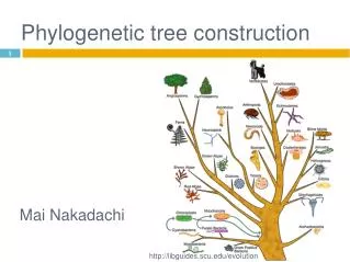
Phylogenetic Tree Reconstruction. Tandy Warnow The Program in Evolutionary Dynamics at Harvard University The University of Texas at Austin. Phylogeny. From the Tree of the Life Website, University of Arizona. Orangutan. Human. Gorilla. Chimpanzee. Reconstructing the “Tree” of Life.

E N D
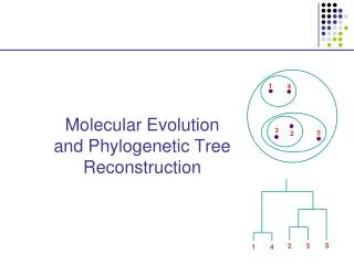
Phylogenetic Tree Reconstruction Tandy Warnow The Program in Evolutionary Dynamics at Harvard University The University of Texas at Austin
Phylogeny From the Tree of the Life Website,University of Arizona Orangutan Human Gorilla Chimpanzee
Reconstructing the “Tree” of Life Handling large datasets: millions of species
Cyber Infrastructure for Phylogenetic Research Purpose: to create a national infrastructure of hardware, algorithms, database technology, etc., necessary to infer the Tree of Life. Group: 40 biologists, computer scientists, and mathematicians from 13 institutions. Funding: $11.6 M (large ITR grant from NSF).
University of New Mexico Bernard Moret David Bader Tiffani Williams UCSD/SDSC Fran Berman Alex Borchers David Stockwell Phil Bourne John Huelsenbeck Mark Miller Michael Alfaro Tracy Zhao University of Connecticut Paul O Lewis University of Pennsylvania Susan Davidson Junhyong Kim Sampath Kannan UT Austin Tandy Warnow David M. Hillis Warren Hunt Robert Jansen Randy Linder Lauren Meyers Daniel Miranker Usman Roshan Luay Nakhleh University of Arizona David R. Maddison University of British Columbia Wayne Maddison North Carolina State University Spencer Muse American Museum of Natural History Ward C. Wheeler UC Berkeley Satish Rao Steve Evans Richard M Karp Brent Mishler Elchanan Mossel Eugene W. Myers Christos M. Papadimitriou Stuart J. Russell SUNY Buffalo William Piel Florida State University David L. Swofford Mark Holder Yale University Michael Donoghue Paul Turner sanofi-aventis Lisa Vawter CIPRes Members
Phylogeny Problem U V W X Y AGGGCAT TAGCCCA TAGACTT TGCACAA TGCGCTT X U Y V W
Steps in a phylogenetic analysis • Gather data • Align sequences • Reconstruct phylogeny on the multiple alignment - often obtaining a large number of trees • Compute consensus (or otherwise estimate the reliable components of the evolutionary history) • Perform post-tree analyses.
CIPRES research in algorithms • Heuristics for NP-hard problems in phylogeny reconstruction • Compact representation of sets of trees • Reticulate evolution reconstruction • Performance of phylogeny reconstruction methods under stochastic models of evolution • Gene order phylogeny • Genomic alignment • Lower bounds for MP • Distance-based reconstruction • Gene family evolution • High-throughput phylogenetic placement • Multiple sequence alignment
-3 mil yrs AAGACTT AAGACTT -2 mil yrs AAGGCCT AAGGCCT AAGGCCT AAGGCCT TGGACTT TGGACTT TGGACTT TGGACTT -1 mil yrs AGGGCAT AGGGCAT AGGGCAT TAGCCCT TAGCCCT TAGCCCT AGCACTT AGCACTT AGCACTT today AGGGCAT TAGCCCA TAGACTT AGCACAA AGCGCTT AGGGCAT TAGCCCA TAGACTT AGCACAA AGCGCTT DNA Sequence Evolution
Markov models of site evolution Simplest (Jukes-Cantor): • The model tree is a pair (T,{p(e)}), where T is a rooted binary tree, and p(e) is the probability of a substitution on the edge e • The state at the root is random • If a site changes on an edge, it changes with equal probability to each of the remaining states • The evolutionary process is Markovian More complex models (such as the General Markov model) are also considered, with little change to the theory.
Phylogeny Reconstruction U V W X Y AGGGCAT TAGCCCA TAGACTT TGCACAA TGCGCTT X U Y V W
Local optimum Cost Global optimum Phylogenetic trees Phylogenetic reconstruction methods • Hill-climbing heuristics for hard optimization criteria (Maximum Parsimony and Maximum Likelihood) • Polynomial time distance-based methods: Neighbor Joining, etc.
Performance criteria • Running time. • Space. • Statistical performance issues (e.g., statistical consistency) with respect to a Markov model of evolution. • “Topological accuracy” with respect to the underlying true tree. Typically studied in simulation. • Accuracy with respect to a particular criterion (e.g. tree length or likelihood score), on real data.
Maximum Parsimony • Input: Set S of n aligned sequences of length k • Output: A phylogenetic tree T • leaf-labeled by sequences in S • additional sequences of length k labeling the internal nodes of T such that is minimized.
Theoretical results • Neighbor Joining is polynomial time, and statistically consistent under typical models of evolution. • Maximum Parsimony is NP-hard, and even exact solutions are not statistically consistent under typical models. • Maximum Likelihood is of unknown computational complexity, but statistically consistent under typical models.
Problems with NJ • Theory: The convergence rate is exponential: the number of sites needed to obtain an accurate reconstruction of the tree with high probability grows exponentially in the evolutionary diameter. • Empirical: NJ has poor performance on datasets with some large leaf-to-leaf distances.
Neighbor joining has poor accuracy on large diameter model trees[Nakhleh et al. ISMB 2001] Simulation study based upon fixed edge lengths, K2P model of evolution, sequence lengths fixed to 1000 nucleotides. Error rates reflect proportion of incorrect edges in inferred trees. 0.8 NJ 0.6 Error Rate 0.4 0.2 0 0 400 800 1200 1600 No. Taxa
Solving NP-hard problems exactly is … unlikely • Number of (unrooted) binary trees on n leaves is (2n-5)!! • If each tree on 1000 taxa could be analyzed in 0.001 seconds, we would find the best tree in 2890 millennia
Local optimum Cost Global optimum Phylogenetic trees Approaches for “solving” MP/ML • Hill-climbing heuristics (which can get stuck in local optima) • Randomized algorithms for getting out of local optima • Approximation algorithms for MP (based upon Steiner Tree approximation algorithms).
How good an MP analysis do we need? • Our research shows that we need to get within 0.01% of optimal (or better even, on large datasets) to return reasonable estimates of the true tree’s “topology”
Datasets Obtained from various researchers and online databases • 1322 lsu rRNA of all organisms • 2000 Eukaryotic rRNA • 2594 rbcL DNA • 4583 Actinobacteria 16s rRNA • 6590 ssu rRNA of all Eukaryotes • 7180 three-domain rRNA • 7322 Firmicutes bacteria 16s rRNA • 8506 three-domain+2org rRNA • 11361 ssu rRNA of all Bacteria • 13921 Proteobacteria 16s rRNA
Problems with current techniques for MP Average MP scores above optimal of best methods at 24 hours across 10 datasets Best current techniques fail to reach 0.01% of optimal at the end of 24 hours, on large datasets
Problems with current techniques for MP Shown here is the performance of the TNT heuristic search for maximum parsimony on a real dataset of almost 14,000 sequences. The required level of accuracy with respect to MP score is no more than 0.01% error (otherwise high topological error results). (“Optimal” here means best score to date, using any method for any amount of time.) Performance of TNT with time
Empirical problems with existing methods • Heuristics for Maximum Parsimony (MP) and Maximum Likelihood (ML) cannot handle large datasets (take too long!) – weneed new heuristics for MP/ML that can analyze large datasets • Polynomial time methods have poor topological accuracy on large datasets – we need better polynomial time methods
“Boosting” phylogeny reconstruction methods • DCMs “boost” the performance of phylogeny reconstruction methods. DCM Base method M DCM-M
DCMs: Divide-and-conquer for improving phylogeny reconstruction
DCMs (Disk-Covering Methods) • DCMs for polynomial time methods improve topological accuracy (empirical observation), and have provable theoretical guarantees under Markov models of evolution • DCMs for hard optimization problems reduce running time needed to achieve good levels of accuracy (empirically observation) • Each DCM is designed by considering the kinds of datasets the base method will do well or poorly on, and these designs are then tested on real and simulated data.
DCM1 Decompositions Input: Set S of sequences, distance matrix d, threshold value 1. Compute threshold graph 2. If the graph is not triangulated, add additional edges to triangulate. DCM1 decomposition : compute the maximal cliques
DCM1-boosting distance-based methods[Nakhleh et al. ISMB 2001] • DCM1-boosting makes distance-based methods more accurate • Theoretical guarantees that DCM1-NJ converges to the true tree from polynomial length sequences 0.8 NJ DCM1-NJ 0.6 Error Rate 0.4 0.2 0 0 400 800 1200 1600 No. Taxa
Major challenge: MP and ML • Maximum Parsimony (MP) and Maximum Likelihood (ML) remain the methods of choice for most systematists • The main challenge here is to make it possible to obtain good solutions to MP or ML in reasonable time periods on large datasets
Maximum Parsimony • Input: Set S of n aligned sequences of length k • Output: A phylogenetic tree T • leaf-labeled by sequences in S • additional sequences of length k labeling the internal nodes of T such that is minimized.
Maximum parsimony (example) • Input: Four sequences • ACT • ACA • GTT • GTA • Question: which of the three trees has the best MP scores?
Maximum Parsimony ACT ACT ACA GTA GTT GTT ACA GTA GTA ACA ACT GTT
Maximum Parsimony ACT ACT ACA GTA GTT GTA ACA ACT 2 1 1 3 3 2 GTT GTT ACA GTA MP score = 7 MP score = 5 GTA ACA ACA GTA 2 1 1 ACT GTT MP score = 4 Optimal MP tree
Optimal labeling can be computed in linear time O(nk) GTA ACA ACA GTA 2 1 1 ACT GTT MP score = 4 Finding the optimal MP tree is NP-hard Maximum Parsimony: computational complexity
Problems with current techniques for MP Even the best of the current methods do not reach 0.01% of “optimal” on large datasetsin 24 hours. (“Optimal” means best score to date, using any method over any amount of time.) Performance of TNT with time
Observations • The best MP heuristics cannot get acceptably good solutions within 24 hours on most of these large datasets. • Datasets of these sizes may need months (or years) of further analysis to reach reasonable solutions. • Apparent convergence can be misleading.
Tree Bisection and Reconnection (TBR) Delete an edge
Tree Bisection and Reconnection (TBR) Reconnect the trees with a new edge that bifurcates an edge in each tree
A conjecture as to why current techniques are poor: • Our studies suggest that trees with near optimal scores tend to be topologically close (RF distance less than 15%) from the other near optimal trees. • The standard technique (TBR) for moving around tree space explores O(n3) trees, which are mostly topologically distant. • So TBR may be useful initially (to reach near optimality) but then more “localized” searches are more productive.
Using DCMs differently • Observation: DCMs make small local changes to the tree • New algorithmic strategy: use DCMs iteratively and/or recursively to improve heuristics on large datasets • However, the initial DCMs for MP • produced large subproblems and • took too long to compute • We needed a decomposition strategy that produces small subproblems quickly.
Using DCMs differently • Observation: DCMs make small local changes to the tree • New algorithmic strategy: use DCMs iteratively and/or recursively to improve heuristics on large datasets • However, the initial DCMs for MP • produced large subproblems and • took too long to compute • We needed a decomposition strategy that produces small subproblems quickly.
Using DCMs differently • Observation: DCMs make small local changes to the tree • New algorithmic strategy: use DCMs iteratively and/or recursively to improve heuristics on large datasets • However, the initial DCMs for MP • produced large subproblems and • took too long to compute • We needed a decomposition strategy that produces small subproblems quickly.
Input: Set S of sequences, and guide-tree T 1. Compute short subtree graph G(S,T), based upon T 2. Find clique separator in the graph G(S,T) and form subproblems New DCM3 decomposition • DCM3 decompositions • can be obtained in O(n) time • (2) yield small subproblems • (3) can be used iteratively
Iterative-DCM3 T DCM3 Base method T’
New DCMs • DCM3 • Compute subproblems using DCM3 decomposition • Apply base method to each subproblem to yield subtrees • Merge subtrees using the Strict Consensus Merger technique • Randomly refine to make it binary • Recursive-DCM3 • Iterative DCM3 • Compute a DCM3 tree • Perform local search and go to step 1 • Recursive-Iterative DCM3