Download
1 / 58
580 likes | 715 Views
Testability. Virendra Singh Indian Institute of Science Bangalore. IEP on Digital System Synthesis At IIT Kanpur. Why Model Faults?. I/O function tests inadequate for manufacturing (functionality versus component and interconnect testing)

E N D
Testability Virendra Singh Indian Institute of Science Bangalore IEP on Digital System Synthesis At IIT Kanpur Testability@IITK
Why Model Faults? • I/O function tests inadequate for manufacturing (functionality versus component and interconnect testing) • Real defects (often mechanical) too numerous and often not analyzable • A fault model identifies targets for testing • A fault model makes analysis possible • Effectiveness measurable by experiments Testability@IITK
Some Real Defects in Chips • Processing defects • Missing contact windows • Parasitic transistors • Oxide breakdown • . . . • Material defects • Bulk defects (cracks, crystal imperfections) • Surface impurities (ion migration) • . . . • Time-dependent failures • Dielectric breakdown • Electromigration • . . . • Packaging failures • Contact degradation • Seal leaks • . . . Ref.: M. J. Howes and D. V. Morgan, Reliability and Degradation - Semiconductor Devices and Circuits, Wiley, 1981. Testability@IITK
Common Fault Models • Single stuck-at faults • Transistor open and short faults • Memory faults • PLA faults (stuck-at, cross-point, bridging) • Functional faults (processors) • Delay faults (transition, path) • Analog faults • For more details of fault models, see M. L. Bushnell and V. D. Agrawal, Essentials of Electronic Testing for Digital, Memory and Mixed-Signal VLSI Circuits, Springer, 2000. Testability@IITK
Single Stuck-at Fault • Three properties define a single stuck-at fault • Only one line is faulty • The faulty line is permanently set to 0 or 1 • The fault can be at an input or output of a gate • Example: XOR circuit has 12 fault sites ( ) and 24 single stuck-at faults Faulty circuit value Good circuit value j c 0(1) s-a-0 d a 1(0) g h 1 z i 0 1 e b 1 k f Test vector for h s-a-0 fault Testability@IITK
Purpose - Testability • Need approximate measure of: • Difficulty of setting internal circuit lines to 0 or 1 by setting primary circuit inputs • Difficulty of observing internal circuit lines by observing primary outputs • Uses: • Analysis of difficulty of testing internal circuit parts – redesign or add special test hardware • Guidance for algorithms computing test patterns – avoid using hard-to-control lines • Estimation of fault coverage • Estimation of test vector length Testability@IITK
Testability Analysis • Involves Circuit Topological analysis, but no test vectors and no search algorithm • Static analysis • Linear computational complexity • Otherwise, is pointless – might as well use automatic test-pattern generation and calculate: • Exact fault coverage • Exact test vectors Testability@IITK
Types of Measures • SCOAP – Sandia Controllability and Observability Analysis Program • Combinational measures: • CC0 – Difficulty of setting circuit line to logic 0 • CC1 – Difficulty of setting circuit line to logic 1 • CO – Difficulty of observing a circuit line • Sequential measures – analogous: • SC0 • SC1 • SO Testability@IITK
Range of SCOAP Measures • Controllabilities – 1 (easiest) to infinity (hardest) • Observabilities – 0 (easiest) to infinity (hardest) • Combinational measures: • Roughly proportional to # circuit lines that must be set to control or observe given line • Sequential measures: • Roughly proportional to # times a flip-flop must be clocked to control or observe given line Testability@IITK
Goldstein’s SCOAP Measures • AND gate O/P 0 controllability: output_controllability = min (input_controllabilities) + 1 • AND gate O/P 1 controllability: output_controllability = S (input_controllabilities) +1 • XOR gate O/P controllability output_controllability = min (controllabilities of each input set) + 1 • Fanout Stem observability: S or min (some or all fanout branch observabilities) Testability@IITK
Controllability Examples Testability@IITK
More ControllabilityExamples Testability@IITK
Observability Examples To observe a gate input: Observe output and make other input values non-controlling Testability@IITK
More Observability Examples To observe a fanout stem: Observe it through branch with best observability Testability@IITK
BIST Motivation • Useful for field test and diagnosis (less expensive than a local automatic test equipment) • Software tests for field test and diagnosis: • Low hardware fault coverage • Low diagnostic resolution • Slow to operate • Hardware BIST benefits: • Lower system test effort • Improved system maintenance and repair • Improved component repair • Better diagnosis Testability@IITK
Costly Test Problems Alleviated by BIST • Increasing chip logic-to-pin ratio – harder observability • Increasingly dense devices and faster clocks • Increasing test generation and application times • Increasing size of test vectors stored in ATE • Expensive ATE needed for 1 GHz clocking chips • Hard testability insertion – designers unfamiliar with gate-level logic, since they design at behavioral level • In-circuit testing no longer technically feasible • Shortage of test engineers • Circuit testing cannot be easily partitioned Testability@IITK
Typical Quality Requirements • 98% single stuck-at fault coverage • 100% interconnect fault coverage • Reject ratio – 1 in 100,000 Testability@IITK
Economics – BIST Costs • Chip area overhead for: • Test controller • Hardware pattern generator • Hardware response compacter • Testing of BIST hardware • Pin overhead -- At least 1 pin needed to activate BIST operation • Performance overhead – extra path delays due to BIST • Yield loss – due to increased chip area or more chips In system because of BIST • Reliability reduction – due to increased area • Increased BIST hardware complexity – happens when BIST hardware is made testable Testability@IITK
BIST Benefits • Faults tested: • Single combinational / sequential stuck-at faults • Delay faults • Single stuck-at faults in BIST hardware • BIST benefits • Reduced testing and maintenance cost • Lower test generation cost • Reduced storage / maintenance of test patterns • Simpler and less expensive ATE • Can test many units in parallel • Shorter test application times • Can test at functional system speed Testability@IITK
Definitions • BILBO – Built-in logic block observer, extra hardware added to flip-flops so they can be reconfigured as an LFSR pattern generator or response compacter, a scan chain, or as flip-flops • Concurrent testing – Testing process that detects faults during normal system operation • CUT – Circuit-under-test • Exhaustive testing – Apply all possible 2npatterns to a circuit with n inputs • Irreducible polynomial – Boolean polynomial that cannot be factored • LFSR – Linear feedback shift register, hardware that generates pseudo-random pattern sequence Testability@IITK
More Definitions • Primitive polynomial – Boolean polynomialp (x)that can be used to compute increasing powersnofxn modulo p (x)to obtain all possible non-zero polynomials of degree less thanp (x) • Pseudo-exhaustive testing – Break circuit into small, overlapping blocks and test each exhaustively • Pseudo-random testing – Algorithmic pattern generator that produces a subset of all possible tests with most of the properties of randomly-generated patterns • Signature – Any statistical circuit property distinguishing between bad and good circuits • TPG – Hardware test pattern generator Testability@IITK
BIST Process • Test controller – Hardware that activates self-test simultaneously on all PCBs • Each board controller activates parallel chip BIST Diagnosis effective only if very high fault coverage Testability@IITK
BIST Architecture • Note: BIST cannot test wires and transistors: • From PI pins to Input MUX • From POs to output pins Testability@IITK
BILBO – Works as Both a PG and a RC • Built-in Logic Block Observer (BILBO) -- 4 modes: • Flip-flop • LFSR pattern generator • LFSR response compacter • Scan chain for flip-flops Testability@IITK
Complex BIST Architecture • Testing epoch I: • LFSR1 generates tests for CUT1 and CUT2 • BILBO2 (LFSR3) compacts CUT1 (CUT2) • Testing epoch II: • BILBO2 generates test patterns for CUT3 • LFSR3 compacts CUT3 response Testability@IITK
Pattern Generation • Store in ROM – too expensive • Exhaustive • Pseudo-exhaustive • Pseudo-random (LFSR) – Preferred method • Binary counters – use more hardware than LFSR • Modified counters • Test pattern augmentation • LFSR combined with a few patterns in ROM • Hardwarediffracter – generates pattern cluster in neighborhood of pattern stored in ROM Testability@IITK
Exhaustive Pattern Generation • Shows that every state and transition works • For n-input circuits, requires all 2n vectors • Impractical for n > 20 Testability@IITK
Pseudo-Exhaustive Method • Partition large circuit into fanin cones • Backtrace from each PO to PIs influencing it • Test fanin cones in parallel • Reduced # of tests from 28 = 256 to 25 x 2 = 64 • Incomplete fault coverage Testability@IITK
Pseudo-Exhaustive Pattern Generation Testability@IITK
Pseudo-Random Pattern Generation • StandardLinear Feedback Shift Register (LFSR) • Produces patterns algorithmically – repeatable • Has most of desirable random # properties • Need not cover all 2n input combinations • Long sequences needed for good fault coverage Testability@IITK
Matrix Equation for Standard LFSR 0 0 . . . 0 0 1 X0 (t + 1) X1 (t + 1) . . . Xn-3 (t + 1) Xn-2 (t + 1) Xn-1 (t + 1) 0 1 . . . 0 0 h2 … … … … … 0 0 . . . 1 0 hn-2 0 0 . . . 0 1 hn-1 X0 (t) X1 (t) . . . Xn-3 (t) Xn-2 (t) Xn-1 (t) 1 0 . . . 0 0 h1 = X (t + 1) = Ts X (t) (Ts is companion matrix) Testability@IITK
Standard n-Stage LFSR Implementation • Autocorrelation – any shifted sequence same as original in 2n-1 – 1 bits, differs in 2n-1 bits • If hi = 0, that XOR gate is deleted Testability@IITK
LFSR Theory • Cannot initialize to all 0’s – hangs • If X is initial state, progresses through states X, Ts X, Ts2 X, Ts3 X, … • Matrix period: Smallest k such that Tsk = I • k LFSR cycle length • Described by characteristic polynomial: f (x) = |Ts – I X | = 1 + h1x + h2x2 + … + hn-1xn-1 + xn Testability@IITK
Example External XOR LFSR • Characteristic polynomial f (x) = 1 + x + x3 (read taps from right to left) Testability@IITK
X0 X1 X2 1 0 0 0 0 1 0 1 0 1 0 1 0 1 1 1 1 1 1 1 0 1 0 0 0 0 1 X0 (t + 1) X1 (t + 1) X2 (t + 1) 0 0 1 1 0 1 0 1 0 X0 (t) X1 (t) X2 (t) = External XOR LFSR • Pattern sequence for example LFSR (earlier): • Always have 1 and xn terms in polynomial • Never repeat an LFSR pattern more than 1 time –Repeats same error vector, cancels fault effect … Testability@IITK
Generic Modular LFSR Testability@IITK
Modular Internal XOR LFSR • Described by companion matrixTm = TsT • Internal XOR LFSR – XOR gates in between D flip-flops • Equivalent to standard External XOR LFSR • With a different state assignment • Faster – usually does not matter • Same amount of hardware • X (t + 1) = Tm x X (t) • f (x) = | Tm – I X | = 1 + h1 x + h2x2 + … + hn-1xn-1 + xn • Right shift – equivalent to multiplying by x, and then dividing by characteristic polynomial and storing the remainder Testability@IITK
Modular LFSR Matrix 0 1 0 . . . 0 0 0 X0 (t + 1) X1 (t + 1) X2 (t + 1) . . . Xn-3 (t + 1) Xn-2 (t + 1) Xn-1 (t + 1) 0 0 1 . . . 0 0 0 0 0 0 . . . 0 0 0 … … … … … … 0 0 0 . . . 0 1 0 0 0 0 . . . 0 0 1 X0 (t) X1 (t) X2 (t) . . . Xn-3 (t) Xn-2 (t) Xn-1 (t) 1 h1 h2 . . . hn-3 hn-2 hn-1 = Testability@IITK
Example Modular LFSR • f (x) = 1 + x2 + x7 + x8 • Read LFSR tap coefficients from left to right Testability@IITK
Primitive Polynomials • Want LFSR to generate all possible 2n – 1 patterns (except the all-0 pattern) • Conditions for this – must have a primitive polynomial: • Monic – coefficient of xn term must be 1 • Modular LFSR – all D FF’s must right shift through XOR’s from X0 through X1, …, through Xn-1, which must feed back directly to X0 • Standard LFSR – all D FF’s must right shift directly from Xn-1 through Xn-2, …, through X0, which must feed back into Xn-1 through XORing feedback network Testability@IITK
Primitive Polynomials (continued) • Characteristic polynomial must divide the polynomial 1 – xk for k = 2n – 1, but not for any smaller k value • See Appendix B of book for tables of primitive polynomials • If p (error) = 0.5, no difference between behavior of primitive & non-primitive polynomial • But p (error) is rarely = 0.5 In that case, non-primitive polynomial LFSR takes much longer to stabilize with random properties than primitive polynomial LFSR Testability@IITK
s-a-0 F Weighted Pseudo-Random Pattern Generation • If p (1) at all PIs is 0.5, pF (1) = 0.58 = • Will need enormous # of random patterns to test a stuck-at 0 fault on F -- LFSR p (1) = 0.5 • We must not use an ordinary LFSR to test this • IBM – holds patents on weighted pseudo-random pattern generator in ATE 1 256 f 1 256 255 256 pF (0) = 1 – = Testability@IITK
Weighted Pseudo-Random Pattern Generator • LFSR p (1) = 0.5 • Solution: Add programmable weight selection and complement LFSR bits to get p (1)’s other than 0.5 • Need 2-3 weight sets for a typical circuit • Weighted pattern generator drastically shortens pattern length for pseudo-random patterns Testability@IITK
w1 0 0 0 0 w2 0 0 1 1 Inv. 0 1 0 1 p (output) ½ ½ ¼ 3/4 w1 1 1 1 1 w2 0 0 1 1 Inv. 0 1 0 1 p (output) 1/8 7/8 1/16 15/16 Weighted Pattern Gen. Testability@IITK
Cellular Automata (CA) • Superior to LFSR – even “more” random • No shift-induced bit value correlation • Can make LFSR more random with linear phase shifter • Regular connections – each cell only connects to local neighbors xc-1 (t) xc (t) xc+1 (t) Gives CA cell connections 111 110 101 100 011 010 001 000 • xc (t + 1) 0 1 0 1 1 0 1 0 26 + 24 + 23 + 21 = 90 Called Rule 90 • xc (t + 1) = xc-1 (t) xc+1 (t) Testability@IITK
Response Compaction • Severe amounts of data in CUT response to LFSR patterns – example: • Generate 5 million random patterns • CUT has 200 outputs • Leads to: 5 million x 200 = 1 billion bits response • Uneconomical to store and check all of these responses on chip • Responses must be compacted Testability@IITK
Definitions • Aliasing – Due to information loss, signatures of good and some bad machines match • Compaction – Drastically reduce # bits in original circuit response – lose information • Compression – Reduce # bits in original circuit response – no information loss – fully invertible (can get back original response) • Signature analysis – Compact good machine response into good machine signature. Actual signature generated during testing, and compared with good machine signature • Transition Count Response Compaction – Count # transitions from 0 1 and 1 0 as a signature Testability@IITK
Transition Counting Testability@IITK
Transition Counting Details • Transition count: C (R) = S (riri-1) for all m primary outputs • To maximize fault coverage: • Make C (R0) – good machine transition count – as large or as small as possible m i = 1 Testability@IITK
LFSR for Response Compaction • Use cyclic redundancy check code (CRCC) generator (LFSR) for response compacter • Treat data bits from circuit POs to be compacted as a decreasing order coefficient polynomial • CRCC divides the PO polynomial by its characteristic polynomial • Leaves remainder of division in LFSR • Must initialize LFSR to seed value (usually 0) before testing • After testing – compare signature in LFSR to known good machine signature • Critical: Must compute good machine signature Testability@IITK