Download
1 / 30
300 likes | 453 Views
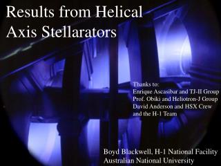
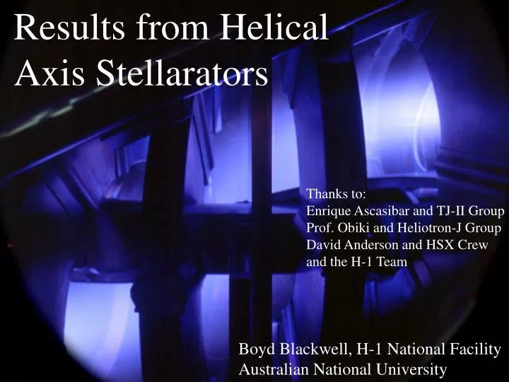
Results from Helical Axis Stellarators. Thanks to: Enrique Ascasibar and TJ-II Group Prof. Obiki and Heliotron-J Group David Anderson and HSX Crew and the H-1 Team. Boyd Blackwell, H-1 National Facility Australian National University. Outline. Brief history Comparative parameters

E N D
Results from Helical Axis Stellarators Thanks to:Enrique Ascasibar and TJ-II GroupProf. Obiki and Heliotron-J GroupDavid Anderson and HSX Crewand the H-1 Team Boyd Blackwell, H-1 National FacilityAustralian National University
Outline Brief history Comparative parameters magnetic surfaces plasma formation and heating diagnostic issues Transport Stability fluctuations Acknowledgements: TJ-II, Heliotron-J, HSX and H-1 groups for their contributions and access to their data, in particular C. Alejaldre, E. Ascasibar, C. Hidalgo, T. Obiki, K. Nagasaki, D.T. Anderson, J.H.Harris, M.G. Shats, J. Howard, Nyima Gyaltsin, S. M. Collis and D.L. Rudakov.
Development of Helical Axis Stellarators Spitzer 1951 - figure-8 stellarator “spatial axis” which produces rotational transform magnetic hill unstable to interchange Koenig 1955 - helical winding/axis: = 1 one pair of helices Spitzer 1956 possibility of shear stabilization for higher order windings = 2,3demonstrated theoretically (resistivity 0) Johnson et al 1958 Furth, Killeen, Rosenbluth 1963found resistive interchange instability possible even at low resistivity for small scale lengths 1964-5 several configurations proposed with magnetic well (average minimum B) found including heliac (straight). Exploitation of avg. min B regions of bad curvature possible ballooning instability -I +I = 1
Development of Helical Axis Stellarators II Nagao 1977Asperator NP: toroidal helical axis stellarator (+extra helical windings) Yoshikawa... 1982-4 - toroidal heliac HX-1 proposal Blackwell, Hamberger... 1984 - SHEILA prototype heliac (0.2M, 0.2T, 1019m3)Harris.. 1985 flexible heliac: = 1 winding varies iota, well over large range 1985 - Tohoku, H-1 and TJ-II and heliacs proposed - and Ribe’s linear heliac UW - Operation in 1987 (Tohoku, Sendai) 1992 (H-1) and 1996(TJ-II, Spain) 1988 Nuhrenberg and Zille - quasi-helical symmetry - restore outstanding features of straight heliac. [transport, beta limit(Monticello et. al 1983)] 1996-9Heliotron-J - combine heliotron/torsatron with advances in transport (optimise bumpy cpt, quasi-isodynamic) 1999 Helically SymmetricEXperiment first quasi-symmetric experiment exploit high iota, N-m scaling
Helical Axis Stellarators 2000 bn,m Canberra, Australia external vacuum vessel CIEMAT, Madrid internal vessel, upgrade to NBI IAE Kyoto “inverted heliac” bumpy field cpt TSL, Madisoncontrolled “spoiling” of symmetry . Device Type Aspect Iota H-1 Heliac3 period heliac, toroidal>helical 5 .15 TJ-II Heliac4 period heliac, helical>toroidal 7 0.9-2.2 Heliotron Jhelical axis heliotron (TFC + =1) 7-11 0.2-0.8 HSXmodular coils, helical symmetry 8 1.05-1.2
Brief history Comparative parameters magnetic surfacesHeliotron J and HSX plasma formation and heating diagnostic issues Transport Stability fluctuations Helical Axis Stellarators 2000 bn,m Canberra, Australia external vacuum vessel CIEMAT, Madrid internal vessel, upgrade to NBI IAE Kyoto “inverted heliac” bumpy field cpt TSL, Madisoncontrolled “spoiling” of symmetry . Device Type Aspect Iota H-1 Heliac3 period heliac, toroidal>helical 5 .15 TJ-II Heliac4 period heliac, helical>toroidal 7 0.9-2.2 Heliotron Jhelical axis heliotron (TFC + =1) 7-11 0.2-0.8 HSXmodular coils, helical symmetry 8 1.05-1.2
Outer Vertical Coil Inner Vertical Coil Vacuum Chamber Toroidal Coil A Toroidal Coil B Plasma Helical Coil Device Parameters of Heliotron J Coil System L=1/M=4 helical coil 0.96MAT Toroidal coil A 0.6MAT Toroidal coil B 0.218MAT Main vertical coil 0.84MAT Inner vertical coil 0.48MAT Major radius 1.2m Minor radius of helical coil 0.28m Vacuum chamber 2.1m3 Aspect ratio 7 Port 65 Magnetic Field 1.5T Pulse length 0.5sec Pitch modulation of helical coil
The Heliotron J Device TFC-A TFC-B HFC Aux.VFC Main VFC
(a) (b) Fig.3 The magnetic surfaces at = 67.5 in the standard configuration. (a) Theexperimental results (corrected) and (b) The calculated magnetic surfaces. Magnetic Surface Mapping STD config, 0.03 Tesla, corrected for earth’s field
Heliotron-J surfaces: cfg “A” - helical divertor Configuration “A” is designed to create a helical divertor region shown in red and yellow. The position of the plasma is shown relative to the helical conductor and the vacuum vessel Other configurations • island divertor • standard from T. Mizuuchi, M. Nakasuga et al. Stellararor Workshop 1999
HSX Parameters Helically Symmetric ExperimentUW, Madison R = 1.2 a=0.15B0=1.3T 4 periodsiota 1.05-1.12 well ~1% essentially 1 term in B0 spect 28GHz@200kWne~3e12 for 50kW@0.5T
HSX Magnetic surfaces Good magnetic surfaces, iota ~ 1% accurate Drift surfaces coincide well with magnetic surfaces - low toroidal effects, high effective iota (eff = N-m)
HSX Magnetic surfaces Good magnetic surfaces, iota ~ 1% accurate Drift surfaces coincide well with magnetic surfaces - low toroidal effects, high effective iota (eff = N-m) Measured drift surfaces mapped to Boozer coordinates Expected drift if fully toroidal
Helical Axis Stellarators 2000 bn,m Canberra, Australia external vacuum vessel CIEMAT, Madrid internal vessel, upgrade to NBI IAE Kyoto “inverted heliac” bumpy field cpt TSL, Madisoncontrolled “spoiling” of symmetry . Device Type Aspect Iota H-1 Heliac3 period heliac, toroidal>helical 5 .15 TJ-II Heliac4 period heliac, helical>toroidal 7 0.9-2.2 Heliotron Jhelical axis heliotron (TFC + =1) 7-11 0.2-0.8 HSXmodular coils, helical symmetry 8 1.05-1.2 Comparative parameters magnetic surfaces plasma formation and heating (H-1, HSX) diagnostic issues Transport
H-1 Heliac: Parameters 3 period heliac: 1992 Major radius 1m Minor radius 0.1-0.2m Vacuum chamber 33m2 excellent access Aspect ratio 5+ toroidal Magnetic Field 1 Tesla (0.2 DC) Heating Power 0.2(0.4)MW GHz ECH 0.3MW 6-25MHz ICH Parameters: achieved / expected n3e18/1e19 T~100eV(Ti)/0.5-1keV(Te) 0.1/0.5%
Complex geometry requires minimum 2D diagnostic H-1 Heliac: Parameters 3 period heliac: 1992 Major radius 1m Minor radius 0.1-0.2m Vacuum chamber 33m2 Aspect ratio 5+ Magnetic Field 1 Tesla (0.2 DC) Heating Power 0.2(0.4)MW GHz ECH 0.3MW 6-25MHz ICH Parameters: achieved / expected n3e18/1e19 T~100eV(Ti)/0.5-1keV(Te) 0.1/0.5% Cross-section of the magnet structure showing a 3x11 channel tomographic diagnostic
2D electron density tomography Helical axis non-circular need true 2D coherent drift mode in argon, 0.08T H density profile evolution (0.5T rf) Raw chordal data Tomographically inverted data
HSX ECH Plasma Utilize 2nd harmonic ECH at 28GHz to examine confinement of deeply-trapped electrons
Plasma production and heating:resonant and non-resonant RF • Non-resonant heating is flexible in B0, works better at low fields. • Resonant heating is much more successful at high fields. <ne> 1018m-3 helicon/frame antenna Magnetic Field (T) = Chon axis
Ion Temperature Camera Intensity temperature rotation Hollow Ti at low B0 radius 0 10 20 30 time (ms)
Helical Axis Stellarators 2000 bn,m Canberra, Australia external vacuum vessel CIEMAT, Madrid internal vessel, upgrade to NBI IAE Kyoto “inverted heliac” bumpy field cpt TSL, Madisoncontrolled “spoiling” of symmetry . Device Type Aspect Iota H-1 Heliac3 period heliac, toroidal>helical 5 .15 TJ-II Heliac4 period heliac, helical>toroidal 7 0.9-2.2 Heliotron Jhelical axis heliotron (TFC + =1) 7-11 0.2-0.8 HSXmodular coils, helical symmetry 8 1.05-1.2 diagnostic issues Transport confinement (Heliotron-J, TJ-II, H-1) Stability/Fluctuations
Fig. 2 Dependence of the diamagnetic stored energy on the magnetic field strength. Heliotron-J: Confinement during ECH • ECH 400kW 53GHZ 50ms • <> ~ 0.2%, <20% radiated • some Fe Ti C O impuritiesPlans: • will upgrade to 70GHz, 500kW • ultimately 4MW ~20kJ? • impurity control • explore bumpiness and hel. divertors Initial Plasma: 700J stored energy W-Diamagnetic vs B is peaked, 700J max
TJ-II Heliac, CIEMAT, Spain Helical/central conductor • R = 1.5 m, a < 0.22 m, 4 periods • B0 < 1.2 T • PECRH < 600 kW from 2 ECH systems • PNBI < 3 MW under installation • helium and hydrogen plasma • Te ~ 2keV, low radiated powers (<20%) • wall desorption rate limits operation in He at P< 600 kW
Thomson scattering • Helium plasmas with injected power of 300 kW • Neoclassical Monte-Carlo agrees well Inferred positive ambipolar Er, confinement time ~ 5ms ~ ISS95yet no serious accumulation of impurities
Configuration Scan (iota) • iota ~ 1.28 – 2.24, up to 1.2 x 10¹⁹ m-3 and 2.0 keV Iota = 2 • When corrected for volume changes, a positive dependence on iota is revealed in helium, (less in H) (tendency sim. to ISS95)
Confinement transitions in H-1 Parameter space map, ~ 1.4 “Pressure” (Is) profile evolution during transition PRF (kW) transition B0(T) • many features in common with large machines • associated with edge shear in Er • easily reproduced and investigated
Bulk Rotation Damped in Heliac 0 0 ExB and ion bulk rotation velocity in high confinement mode: magnetic structure causes viscous damping of rotation Radial force balance Vp, Vt << VExB ~ 1/(neB) dPi/dr Mass (ion) flow velocities much smaller than corresponding VExB
diagnostic issues Transport Stability fluctuations Issues: Interchange and Ballooning Modes (DTEM low ) Tools: Configuration Flexibility e.g. transform and magnetic well (even hill!) First Impression: No unworkable instabilties or disruptions “Drift-like” instability in H-1 at low field • Triple-Mach-Triple probe • disappears as B increases Helical axis high iota short connection lengthAll devices need > 0.5-1% to test ballooning stability
TJ-II Turbulence/Fluctuation studies • ExB sheared flows observed near edge rational surfaces (8/5, 4/2) • Spectra mainly <200kHz, 10-40% (edge?), correlation time 10ms • MHD (ELM-like) events (for W~1kJ) - magnetic activity - spike in the Ha signal. • Fluctuations increase with magnetic hill near edge • resistive ballooning?
Summary - Future • Confinement in heliacs ~ISS95 or better (2keV, ~5ms). Ion beam probe to elucidate role of Eradial in improved confinement • New configurations with improved neoclassical transport initial results promising, await mature data, analysis • HSX/H-J can compare similar configurations with vastly different neoclassical transport predictions. • Confinement transitions possible at low power, many similarities with large devices/powers. Investigate effect of E-field imposed by localised ECH. • No serious impurity accumulation problems yet. Real test when the ions are strongly heated • No fatal instabilities observed yet. Several devices should have the heating capacity to test ballooning limits, at least in degraded configurations (consequence of flexibility).