C onjugate gradients, sparse matrix-vector multiplication, and graph partitioning

1. Conjugate gradients, sparse matrix-vector multiplication, and graph partitioning Thanks to AydinBuluc, UmitCatalyurek, Alan Edelman, and Kathy Yelickfor some of these slides.

2. The middleware of scientific computing Continuousphysical modeling Ax = b Linear algebra Computers

3. Example: The Temperature Problem • A cabin in the snow • Wall temperature is 0°, except for a radiator at 100° • What is the temperature in the interior?

4. Example: The Temperature Problem • A cabin in the snow (a square region ) • Wall temperature is 0°, except for a radiator at 100° • What is the temperature in the interior?

5. The physics: Poisson’s equation

6. Many Physical Models Use Stencil Computations • PDE models of heat, fluids, structures, … • Weather, airplanes, bridges, bones, … • Game of Life • many, many others 6.43

7. Examples of stencils 9-point stencil in 2D(game of Life) 5-point stencil in 2D (temperature problem) 25-point stencil in 3D (seismic modeling) 7-point stencil in 3D(3D temperature problem) … and many more

8. Model Problem: Solving Poisson’s equation for temperature • Discrete approximation to Poisson’s equation: x(i) = ¼ ( x(i-k) + x(i-1) + x(i+1) + x(i+k) ) • Intuitively: Temperature at a point is the average of the temperatures at surrounding points k = n1/2

9. Model Problem: Solving Poisson’s equation for temperature • For each i from 1 to n, except on the boundaries: –x(i-k) –x(i-1) + 4*x(i) –x(i+1) –x(i+k) = 0 • n equations in n unknowns: A*x = b • Each row of A has at most 5 nonzeros • In three dimensions, k = n1/3 and each row has at most 7 nzs k = n1/2

10. A Stencil Computation Solves a System of Linear Equations • Solve Ax = b for x • Matrix A, right-hand side vector b, unknown vector x • A is sparse: most of the entries are 0

11. Gaussian elimination Iterative More General Any matrix Symmetric positive definite matrix More Robust The Landscape of Ax = b Algorithms More Robust Less Storage

12. Conjugate gradient iteration to solve A*x=b x0 = 0, r0 = b, d0 = r0 (these are all vectors) for k = 1, 2, 3, . . . αk = (rTk-1rk-1) / (dTk-1Adk-1) step length xk= xk-1 + αk dk-1 approximate solution rk = rk-1 – αk Adk-1 residual = b - Axk βk = (rTkrk) / (rTk-1rk-1) improvement dk= rk+ βk dk-1 search direction • One matrix-vector multiplication per iteration • Two vector dot products per iteration • Four n-vectors of working storage

13. Conjugate gradient primitives • DAXPY: v = α*v + β*w (vectors v, w; scalars α, β) • Almost embarrassingly parallel • DDOT: α = vT*w (vectors v, w; scalar α) • Global sum reduction; span = log n • Matvec: v = A*w (matrix A, vectors v, w) • The hard part • But all you need is a subroutine to compute v from w • Sometimes you don’t need to store A! (e.g. temperature problem) • Usually you do need to store A, but it’s sparse ...

14. Data structure for sparse matrix A (stored by rows) • Full matrix: • 2-dimensional array of real or complex numbers • (nrows*ncols) memory • Sparse matrix: • compressed row storage • about (2*nzs + nrows) memory

15. Distributed-memory sparse matrix data structure P0 P1 • Each processor stores: • # of local nonzeros • range of local rows • nonzeros in CSR form P2 Pn

16. Parallel Dense Matrix-Vector Product (Review) P0 P1 P2 P3 • y = A*x, where A is a dense matrix • Layout: • 1D by rows • Algorithm: Foreach processor j Broadcast X(j) Compute A(p)*x(j) • A(i) is the n by n/p block row that processor Pi owns • Algorithm uses the formula Y(i) = A(i)*X = Sj A(i)*X(j) x P0 P1 P2 P3 y

17. P0 P1 P2 P3 x P0 P1 P2 P3 y Parallel sparse matrix-vector product • Lay out matrix and vectors by rows • y(i) = sum(A(i,j)*x(j)) • Only compute terms with A(i,j) ≠ 0 • Algorithm Each processor i: Broadcast x(i) Compute y(i) = A(i,:)*x • Optimizations • Only send each proc the parts of x it needs, to reduce comm • Reorder matrix for better locality by graph partitioning • Worry about balancing number of nonzeros / processor, if rows have very different nonzero counts

18. Other memory layouts for matrix-vector product • Column layout of the matrix eliminates the broadcast • But adds a reduction to update the destination – same total comm • Blocked layout uses a broadcast and reduction, both on only sqrt(p) processors – less total comm • Blocked layout has advantages in multicore / Cilk++ too P0 P1 P2 P3 P0 P1 P2 P3 P4 P5 P6 P7 P8 P9 P10 P11 P12 P13 P14 P15

19. Graphs and Sparse Matrices • Sparse matrix is a representation of a (sparse) graph 1 2 3 4 5 6 1 1 1 2 1 1 1 3 1 11 4 1 1 5 1 1 6 1 1 3 2 4 1 5 6 • Matrix entries are edge weights • Number of nonzeros per row is the vertex degree • Edges represent data dependencies in matrix-vector multiplication

20. Irregular mesh: NASA Airfoil in 2D

21. Composite Mesh from a Mechanical Structure

22. Converting the Mesh to a Matrix

23. Adaptive Mesh Refinement (AMR) • Adaptive mesh around an explosion • Refinement done by calculating errors

24. Adaptive Mesh fluid density Shock waves in a gas dynamics using AMR (Adaptive Mesh Refinement) See: http://www.llnl.gov/CASC/SAMRAI/

25. Irregular mesh: Tapered Tube (Multigrid)

26. Graphs and Sparse Matrices • Sparse matrix is a representation of a (sparse) graph 1 2 3 4 5 6 1 1 1 2 1 1 1 3 1 11 4 1 1 5 1 1 6 1 1 3 2 4 1 5 6 • Matrix entries are edge weights • Number of nonzeros per row is the vertex degree • Edges represent data dependencies in matrix-vector multiplication

27. Sparse Matrix Vector Multiplication

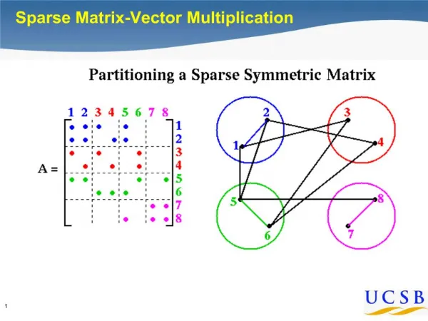
28. edge crossings = 6 edge crossings = 10 Graph partitioning • Assigns subgraphs to processors • Determines parallelism and locality. • Tries to make subgraphs all same size (load balance) • Tries to minimize edge crossings (communication). • Exact minimization is NP-complete.

29. Parallelizing Stencil Computations • Parallelism is simple • Grid is a regular data structure • Even decomposition across processors gives load balance • Spatial locality limits communication cost • Communicate only boundary values from neighboring patches • Communication volume • v = total # of boundary cells between patches

30. Two-dimensional block decomposition • n mesh cells, p processors • Each processor has a patch of n/p cells • Block row (or block col) layout: v = 2 * p * sqrt(n) • 2-dimensional block layout: v = 4 * sqrt(p) * sqrt(n)

31. 2 (2) 1 3 (1) 4 1 (2) 2 4 (3) 3 1 2 2 5 (1) 8 (1) 1 6 5 6 (2) 7 (3) Definition of Graph Partitioning • Given a graph G = (N, E, WN, WE) • N = nodes (or vertices), • E = edges • WN = node weights • WE = edge weights • Often nodes are tasks, edges are communication, weights are costs • Choose a partition N = N1 U N2 U … U NP such that • Total weight of nodes in each part is “about the same” • Total weight of edges connecting nodes in different parts is small • Balance the work load, while minimizing communication • Special case of N = N1 U N2: Graph Bisection

32. Applications • Telephone network design • Original application, algorithm due to Kernighan • Load Balancing while Minimizing Communication • Sparse Matrix times Vector Multiplication • Solving PDEs • N = {1,…,n}, (j,k) in E if A(j,k) nonzero, • WN(j) = #nonzeros in row j, WE(j,k) = 1 • VLSI Layout • N = {units on chip}, E = {wires}, WE(j,k) = wire length • Sparse Gaussian Elimination • Used to reorder rows and columns to increase parallelism, and to decrease “fill-in” • Data mining and clustering • Physical Mapping of DNA

33. Partitioning by Repeated Bisection • To partition into 2k parts, bisect graph recursively k times