Download
1 / 15

E N D
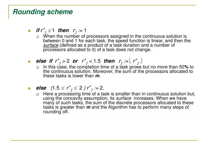
Rounding scheme • ifr*j 1thenrj:= 1 • When the number of processors assigned in the continuous solution is between 0 and 1 for each task, the speed function is linear, and then the surface (defined as a product of a task duration and a number of processors allocated to it)of a task does not change. • elseifr*j > 2orr*j < 1.5then rj:= r*j • In this case, the completion time of a task grows but no more than 50% to the continuous solution. Moreover, the sum of the processors allocated to these tasks is lower than m. • else(1.5r*j2 ) r*j:= 2. • Here a processing time of a task is smaller than in continuous solution but, using the concavity assumption, its surface increases. When we have many of such tasks, the sum of the discrete processors allocated to these tasks is greater than m and the Algorithm has to perform many steps of rounding off.
Algorithm • calculate the C*cont and the optimal continuous processor allocations r*j • round the continuous allocation of processors to the integer valuesrj • calculate the new processing times of the tasks and schedule them in non-increasing order of processing times in parallel (whenever possible use a sequential mode too) • m = rj (j=1,...,n) (a discrete number of processors) • C = max(Cj) • if m = m thenGoToEnd; • whilem < m do allocate an excess of processors to the longest task – GoToEnd • take the minimum value of the schedule length constructed by A or B: • A :whilem > m do • reduce by one a number of processors assigned to the task (group of tasks) with the largest number of processors allotted and assign the tasks that were assigned to excess processors to the released processor and to the other processors if necessary, not exceedingC. • B:tasks assigned to excess processors schedule after the tasks already scheduled treating them as a new instance of the problem. • EndC’max :=C
Example • Let us consider the following data: • n=6, m=4, T= {T1, T2, …, T6}, • t(1) = [32, 34, 14, 92, 18, 55], • f(r) = r, the same for each task. • C*cont= 64.46, • r*= [0.49; 0.53; 0.22; 1.63; 0.28; 0.85]. • From this solution we proceed according to the rounding algorithm. C*cont=64,46 t3(1)=14 t5(1)=18 t1(1)=32 4 t2(1)=34 t4(2)=54,7 processors t6(1)=55 time
C*cont=64,46 t3(1)=14 t1(1)=32 4 t2(1)=34 t5(1)=18 t4(2)=54,7 processors t6(1)=55 time
C*cont=64,46 t3(1)=14 t1(1)=32 4 t2(1)=34 t5(1)=18 t4(2)=54,7 processors t6(1)=55 time
Step A C*cont=64,46 t3(1)=14 t1(1)=32 4 t2(1)=34 t5(1)=18 processors t4(1)=92 t6(1)=55 time
Step A C*cont=64,46 4 t3(1)=14 t1(1)=32 t2(1)=34 t5(1)=18 processors t4(1)=92 t6(1)=55 time
Step B C*cont=64,46 t3(1)=14 t1(1)=32 4 t2(1)=34 t5(1)=18 t4(2)=54,7 processors t6(1)=55 time
Step B Tasks of new instance t1(1)=32 C*cont=64,46 t3(1)=14 4 t2(1)=34 t5(1)=18 t4(2)=54,7 processors t6(1)=55 time
Step B Tasks of new instance C*cont=64,46 4 t2(1)=34 t5(1)=18 t1(3)=14,04 t4(2)=54,7 processors t6(1)=55 t3(1)=14 time
Computational experiments To evaluate the mean behavior of Algorithm we use the following measure: Relative error = C’max / C*cont where • C’max – schedule length obtained by Algorithm • C*cont – optimal schedule length of the continuous solution • Task processing times ti(1) have been generated from a uniform distribution in interval [1, 100]. • Processing speed functions have been chosen as fi(r) = ra, 0 < a 1 • Each entry in the table is a mean value for 25 instances randomly generated.
Average behavior of the Algorithm for different shapes of processing speed functions and varying number of processors
Conclusion • The berth and crane allocation as moldable tasks scheduling problem has been considered. • Starting from the continuous version of the problem (i.e. where the tasks may require a fractional part of the resources), we proposed asuboptimalalgorithm with a very good average behavior. • Further investigations in this area will take into account a construction of the algorithm with a good average and worst case performance guarantee for arbitrary non-decreasing processing speed function.