image, one quantity of interest is the variance: (4)

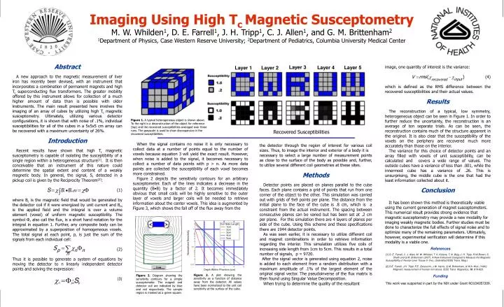
1. Imaging Using High Tc Magnetic SusceptometryM. W. Whilden1, D. E. Farrell1, J. H. Tripp1, C. J. Allen1, and G. M. Brittenham21Department of Physics, Case Western Reserve University; 2Department of Pediatrics, Columbia University Medical Center Abstract A new approach to the magnetic measurement of liver iron has recently been devised, with an instrument that incorporates a combination of permanent magnets and high Tc superconducting flux transformers. The greater mobility offered by this instrument allows for collection of a much higher amount of data than is possible with older instruments. The main result presented here involves the imaging of an array of cubes by utilizing high Tc magnetic susceptometry. Ultimately, utilizing various detector configurations, it is shown that with noise of .1%, individual susceptibilities for all of the cubes in a 5x5x5 cm array can be recovered with a maximum uncertainty of 26%. Introduction Recent results have shown that high Tc magnetic susceptometry is capable of isolating the susceptibility of a single region within a heterogeneous structure[1]. It is then conceivable that an instrument of this nature could determine the spatial extent and content of a weakly magnetic body. In general, the signal, S, detected in a pickup coil is given by the Reciprocity Theorem[2]: (1) where Bc is the magnetic field that would be generated by the detector coil if it were energized by unit current and Bm is the applied field and the integral is over a volume element (voxel) of uniform magnetic susceptibility. The symbol Φ, also call the flux, is a short hand notation for the integral in equation 1. Further, any composite body can be approximated by a superposition of homogeneous voxels. The total signal at each point, p, is just the sum of the signals from each individual cell: (2) Thus it is possible to generate a system of equations by moving the detector to n linearly independent detector points and solving the expression: (3) Layer 3 image, one quantity of interest is the variance: (4) which is defined as the RMS difference between the recovered susceptibilities and their actual values. Results The reconstruction of a typical, low symmetry, heterogeneous object can be seen in Figure 1. In order to further reduce the uncertainty, the reconstruction is an average of ten separate trials. As can be seen, the reconstruction contains much of the structure apparent in the original. It is also clear that the susceptibility of the voxels on the periphery are recovered much more accurately than those on the interior. The variance for this choice of detector points and an array filled with voxels of unit susceptibility, can be calculated and covers a wide range of values. The outside cubes have a variance of less than .001, while the innermost cube has a variance of .26. This is unsurprising, the middle cube is the one that had the least information collected about it. Conclusion It has been shown this method is theoretically viable using the current generation of magnet susceptometers. This numerical result provides strong evidence that magnetic susceptometry may provide a new modality for imaging weakly magnetic bodies. Further studies must be done to characterize the full effects of signal noise and to optimize many of the remaining parameters. Ultimately, however, experimental verification will determine if this modality is a viable one. Layer 4 Layer 5 Layer 1 Layer 2 Figure 1. A typical heterogeneous object is shown above. To the right is a deconstruction of the object for reference (top) and the recovered susceptibilities averaged over three runs. The grayscale is used to show discrepancies in the recovered susceptibilities. Recovered Susceptibilities When the signal contains no noise it is only necessary to collect data at a number of points equal to the number of voxels because equation 3 will yield the exact result. However, when noise is added to the signal, it becomes necessary to collect a number of data points with p > n. As more data points are collected the susceptibility of each voxel becomes more constrained. Figure 2 depicts the sensitivity contours for an arbitrary susceptometer. Each of the lines indicates a decrease in the quantity (B•B) by a factor of 2. It becomes immediately obvious that small coils will be highly sensitive to the outer layer of voxels and larger coils will be needed to retrieve information about the center voxels. This idea is augmented by Figure 3, which shows the fall off of the flux away from the the detector through the region of interest for various coil sizes. Thus, to image the interior and exterior of a body it is necessary to select a large number of measurement points as close to the surface of the body as possible and, further, to utilize several different coil geometries at these sites. Methods Detector points are placed on planes parallel to the cube faces. Each plane contains a grid of points that run from one corner of the object to the other. This simulation was carried out with grids of 9x9 points per plane. The distance from the initial plane to the face of the cube is .8 cm, which is a constraint from the actual instrument. The spacing between consecutive planes can be varied but has been set at .2 cm per plane. For this simulation there are 4 layers of planes per side of the cube. Using this scheme and these specifications there are 1944 detector points. As was seen earlier, it is necessary to utilize different coil and magnet combinations in order to retrieve information regarding the interior. This simulation utilizes five coils of increasing side length from 1cm to 5cm. This results in a total number of signals, p = 9720. After the signal vector is generated using equation 2, noise is added to each element from a random distribution with a maximum amplitude of .1% of the largest element of the original signal vector. The pseudoinverse of the flux matrix is then found using Singular Value Decomposition. When trying to determine the quality of the resultant References [1] D. E. Farrell, C. J. Allen, M. W. Whilden, T. K. Kidane, T. N. Baig, J. H. Tripp, R.W Brown, S. Sheth and G.M. Brittenham (2007). A New Instrument Designed to Measure the Magnetic Susceptibility of Human Liver Tissue In Vivo. (Submitted IEEE Trans. Mag.) [2] D.E. Farrell, J.H. Tripp, P.E. Zanzucchi, J.W. Harris, G.M. Brittenham, & W.A. Muir, (1980). Magnetic measurement of human iron stores. IEEE Trans. Magnetics, 16: 818-823. Funding This work was supported in part by the NIH under Grant RO1DK057209. Figure 3. A plot showing the sensitivity as a function of distance away from the detector. All values have been normalized to the unit coil sensitivity at the surface of the cube. Figure 2. Diagram showing the sensitivity contours for a simple susceptometer. The magnet and detector coil are indicated by blue and red respectively. The sample region is marked as a green square.