Download
1 / 45
450 likes | 452 Views
New uses of remote sensing to understand boundary layer clouds. Rob Wood Jan 22, 2004 Contributions from Kim Comstock, Chris Bretherton, Peter Caldwell, Martin Köhler, Rene Garreaud, and Ricardo Muñoz. Outline. What is remote sensing? Recent work at UW: Pockets of open cells

E N D
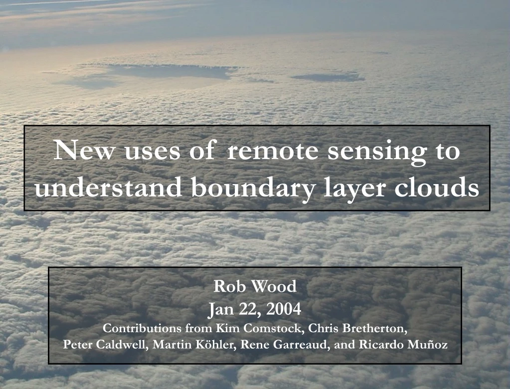
New uses of remote sensing to understand boundary layer clouds Rob Wood Jan 22, 2004 Contributions from Kim Comstock, Chris Bretherton, Peter Caldwell, Martin Köhler, Rene Garreaud, and Ricardo Muñoz
Outline What is remote sensing? Recent work at UW: Pockets of open cells Estimating MBL properties from combined satellite/reanalysis Other new technology What’s next?
What is remote sensing? • Definition: The science, technology and art of obtaining information about objects or phenomena from a distance (i.e., without being in physical contact with them). • Examples: Radar, lidar, all satellite observations Ms. Evelyn Pruitt of the United States Office of Naval Research coined the term “remote sensing” in 1958 to include aerial photography, satellite-based imaging, and other forms of remote data collection.
Recent work at UW • The mystery of open cell pockets • Inferring MBL structure by combining knowledge from satellites and reanalysis
Scanning radars used to observe drizzle from shallow MBL cloud • Scanning C-band (5 cm) radar employed during TEPPS (NE Pacific) and EPIC 2001 (SE Pacific). • Distinct cellular nature of drizzle imaged for the first time • Allows investigation of links between cloud and drizzle structure
C-band radar movie from EPIC 40 km Wind
30 dBZ 20 10 0 -10 60 km 60 km 0235 0250 0305 0320 0335 Structure and evolution of drizzle cells C-band example October 21 0305 LT
Lifetime of drizzle cells/events • Typical cell lifetimes 1-2 hours Mean cloud base rain rates of 0.2-1.0 mm hr-1Cloud liquid water depletion rates do not exceed 0.2 mm hr-1 zi(u.qT)~1 mm hr-1Mesoscale gradients in qTare ~1 g kg-1 over 5-10 km Typical mesoscale u variations must be 1-2 m s-1
C-band reflectivity and radial velocity Mesoscale wind fluctuations related to drizzle cells Radial velocity fluctuations Radar reflectivity
The “POCS” mystery Pockets Of Open Cells (POCS) are frequently observed in otherwise unbroken Sc.Their cause is unknown POCS
The first satellite remote sensor - Tiros 1 TV Camera in space Mesoscale cellular convection
100km MODIS 250m visible imagery
0 Tb 5 Low Tb indicative of low re 11 - 3.75 m brightness temperature difference POCS associated with clean clouds Figure courtesy Bjorn Stevens, UCLA
POCS regions drizzle more Figure by Kim Comstock/Rob Wood
More vigorous drizzle in POCS MODIS brightness temperature difference, GOES thermal IR, scanning C-band radar Figure by Sandra Yuter/Rob Wood
DYCOMS II aircraft mm radar Figure by Bjorn Stevens
POCS and drizzle – summary • POCS are often associated with small cloud effective radius and enhanced drizzle (no counter examples found to date) • Differences in LWP pdf shape are not expected to strongly modulate mean drizzle rate (LWP more skewed in POCS, but with lower cloud fraction) • Drizzle much more heterogeneous in POCS which may cause large horizontal temperature gradients through evaporative cooling – this in turn leads to density currents (“mini cold pools”) that enhance mesoscale fluxes of moisture and energy
MBL depth, entrainment and decoupling • Integrative approach to derive MBL and cloud properties in regions of low cloud • Combines observations from MODIS and TMI with reanalysis from NCEP and climatology from COADS • Results in estimates of MBL depth and decoupling (and climatology of entrainment)
Methodology • Independent observables: LWP, Ttop, SST • Unknowns: zi, q (= ) • Use COADS climatological surface RH and air-sea temperature difference • Use NCEP reanalysis free-tropospheric temperature and moisture • Iterative solution employed to resulting non-linear equation for zi
Mean MBL depth (Sep/Oct 2000) NE Pacific SE Pacific
Mean decoupling parameter q Decoupling scales well with MBL depth
Deriving mean entrainment rates • Use equation: we=uzi+ws • Estimate ws from NCEP reanalysis • Estimate uzifrom NCEP winds and two month mean zi
Mean entrainment rates Entrainment rate [mm/s]◄ NE PacificSE Pacific ►Subsidence rate [mm/s]
Summary of MBL depth work • Scene-by-scene estimation of MBL depth and decoupling • Climatology of entrainment rates over the subtropical cloud regions derived using MBL depth and subsidence from reanalysis • Decoupling strong function of MBL depth • Next step: deriving links between turbulence, inversion strength and entrainment by coupling to simple model forced with realistic boundary conditions
New technology: Multi-angle imaging (MISR) On Terra (launched late 1999)9 cameras in fore and aft direction (-70 to +70)Unprecedented 3D examination of cloud structure
Example of MISR’s potential • Movie
What’s next for MBL cloud remote sensing? SPACEBORNE • millimeter RADAR in space: CLOUDSAT [launch 2004]; EARTHCARE [ESA, launch 2008] first spaceborne drizzle measurements • Cloud/aerosol LIDAR: CALIPSO [launch 2004]; +EARTHCARE MBL aerosol characteristic in clear regions; first direct measurements of MBL depth at high spatial resolution from space GROUND BASED • Scanning MM radars – 3D cloud structure • Scanning LIDAR on aircraft – cloud top mapping and entrainment processes
From Wood et al. (2002) Diurnal cycle –The view from space SE Pacific has similar mean LWP, but much stronger diurnal cycle, than NE Pacific….…Why?A=LWP amplitude/LWP mean
0.05 cm s-1 zi/t + u•zi= we - ws NIGHT DAY NIGHT DAY we dzi/dt ws EPIC 2001 [85W, 20S]Diurnal cycle of subsidencews, entrainmentwe, andzi/t swe=0.24cm s-1 sws=0.26 cm s-1 szi/t=0.44 cm s-1 Conclusion: Subsidence and entrainment contribute equally to diurnal cycle of MBL depth
Quikscat mean and diurnal divergence • Mean divergence observed over most of SE Pacific Coastal SE Peru • Diurnal difference (6L-18L) anomaly off Peruvian/Chilean coast (cf with other coasts) • Anomaly consistent with reduced subsidence (upsidence) in coastal regions at 18L Mean divergence Diurnal difference (6L-18L)
Diurnal subsidence wave - ECMWF • Daytime dry heating leads to ascent over S American continent • Diurnal wave of large-scale ascent propagates westwards over the SE Pacific at 30-50 m s-1 • Amplitude 0.3-0.5 cm s-1• Reaches over 1000 km from the coast, reaching 90W around 15 hr after leaving coast
Subsidence wave in MM5 runs (Garreaud & Muñoz 2003, Universidad de Chile) • Vertical large scale wind at 800 hPa (from 15-day regional MM5 simulation, October 2001) Subsidence prevails over much of the SE Pacific during morning and afternoon (10-18 UTC) A narrow band of strong ascending motion originates along the continental coast after local noon (18 UTC) and propagates oceanward over the following 12 hours, reaching as far west as the IMET buoy (85W, 20S) by local midnight.
Vertical-local time contours (MM5) 17S-73W 22S-71W 21S-76W Height [m] • Vertical wind as a function of height and local time of day – contours every 0.5 cm/s, with negative values as dashed lines Vertical extent of propagating wave limited to < 5-6 km Ascent peaks later further out into the SE Pacific
Diurnal amplitude equal to or exceeds synoptic variability (here demonstrated using 800 hPa potential temperature variability) over much of the SE Pacific, making the diurnal cycle of subsidence a particularly important mode of variability Diurnal vs. synoptic variability (MM5)
22-18S, 78-74W • Wave amplitude greatest during austral summer when surface heating over S America is strongest. Effect present all year round, consistent with dry heating rather than having a deep convective origin MM5 simulations broadly consistent with ECMWF reanalysis data Seasonal cycle of subsidence wave (MM5)
Effect of subsidence diurnal cycle upon cloud properties and radiation • Use mixed layer model (MLM) to attempt to simulate diurnal cycle during EPIC 2001 using: (a) diurnally varying forcings including subsidence rate (b) diurnally varying forcings but constant (mean) subsidence • Compare results to quantify effect of the “subsidence wave” upon clouds, MBL properties, and radiative budgets
MLM results • Entrainment closure from Nicholls and Turton – results agree favourably with observationally-estimated valuesCloud thickness and LWP from both MLM runs higher than observed – stronger diurnal cycle in varying subsidence run. Marked difference in MLM TOA shortwave flux during daytime (up to 10 W m-2, with mean difference of 2.3 W m-2)Longwave fluxes only slightly different (due to slightly different cloud top temperature) Results probably underestimate climatological effect of diurnally-varying subsidence because MLM cannot simulate daytime decoupling SW LW
Conclusions • Reanalysis data and MM5 model runs show a diurnally-modulated 5-6 km deep gravity wave propagating over the SE Pacific Ocean at 30-50 m s-1. The wave is generated by dry heating over the Andean S America and is present year-round. Data are consistent with Quikscat anomaly. • MM5 simulations show the wave to be characterized by a long, but narrow (few hundred kilometers wide) region of upward motion (“upsidence”) passing through a region largely dominated by subsidence. • The wave causes remarkable diurnal modulation in the subsidence rate atop the MBL even at distances of over 1000 km from the coast. • At 85W, 20S, the wave is almost in phase with the diurnal cycle of entrainment rate, leading to an accentuated diurnal cycle of MBL depth, which mixed layer model results show will lead to a stronger diurnal cycle of cloud thickness and LWP. • The wave may be partly responsible for the enhanced diurnal cycle of cloud LWP in the SE Pacific (seen in satellite studies).
Acknowledgements We thank Chris Fairall, Taneil Uttal, and other NOAA staff for the collection of the EPIC 2001 observational data on the RV Ronald H Brown. The work was funded by NSF grant ATM-0082384 and NASA grant NAG5S-10624. References Bretherton, C. S., Uttal, T., Fairall, C. W., Yuter, S. E., Weller, R. A., Baumgardner, D., Comstock, K., Wood, R., 2003: The EPIC 2001 Stratocumulus Study, Bull. Am. Meteorol. Soc., submitted 1/03. Garreaud, R. D., and Muñoz, R., 2003: The dirnal cycle in circulation and cloudiness over the subtropical Southeast Pacific, submitted to J. Clim., 7/03. Wood, R., Bretherton, C. S., and Hartmann, D. L., 2002: Diurnal cycle of liquid water path over the subtropical and tropical oceans. Geophys. Res. Lett.10.1029/2002GL015371, 2002
Ground based radar • Developed during WWII for aircraft detection • Operators surprised by unusual signals that turned out to be caused by rain • Post-WWII: A remote sensing industry is born