Lecture 11: Particles in Finite Potential Wells

“All of modern physics is governed by that magnificent and thoroughly confusing discipline called quantum mechanics...It has survived all tests and there is no reason to believe that there is any flaw in it….We all know how to use it and how to apply it to problems; and so we have learned to live with the fact that nobody can understand it.” --Murray Gell-Mann

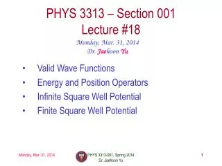
U(x)y(x) U0 n=2 n=1 n=4 n=3 AlGaAs GaAs AlGaAs I II III U(x) 0 L x Lecture 11:Particles in Finite Potential Wells

This week and last week are critical for the course: Week 3, Lectures 7-9: Week 4, Lectures 10-12: Light as Particles Schrödinger Equation Particles as waves Particles in infinite wells, finite wells Probability Uncertainty Principle Midterm Exam Monday, Feb. 13. It will cover lectures 1-11 and some aspects of lectures 11-12.Practice exams: Old exams are linked from the course web page.Review Sunday, Feb. 12, 3-5 PM in 141 Loomis. Office hours: Feb. 12 and 13 Next week:Homework 4 covers material in lecture 10 – due on Thur. Feb. 16.We strongly encourage you to look at the homework before the midterm!Discussion: Covers material in lectures 10-12. There will be a quiz. Lab:Go to 257 Loomis (a computer room). You can save a lot of time by reading the lab ahead of time – It’s a tutorial on how to draw wave functions.

Schrodinger’s Equation (SEQ) A wave equation that describes spatial and time dependence of Y(x,t). Expresses KE +PE = Etot Second derivative extracts -k2 from wave function. Constraints that y(x) must satisfy Existence of derivatives (implies continuity). Boundary conditions at interfaces. Infinitely deep 1D square well (“box”) Boundary conditions y(x) = Nsin(kx), where k = np/L. Discrete energy spectrum: En = n2E1, where E1 = h2/8mL2. Normalization: N = (2/L). Last Time

“Normalizing” the wave function General properties of bound-state wave functions Particle in a finite square well potential Solving boundary conditions Comparison with infinite-well potential Today Midterm material ends here.

electron y(x) n=2 n=1 n=3 x 0 L U =  U =  En n=3 n=2 n=1 0 x L Particle in Infinite Square Well Potential The discrete En are known as “energy eigenvalues”:

y(x)2 corresponds to a physically meaningful quantity: the probability density of finding the particle near x. To avoid unphysical behavior, y(x) must satisfy some conditions: y(x) must be single-valued, and finite. Finite to avoid infinite probability density. y(x) must be continuous, with finite dy/dx. dy/dx is related to the momentum.In regions with finite potential, d2y/dx2 must be finite. To avoid infinite energies. This also means that dy/dxmust be continuous. There is no significance to the overall sign of y(x). It goes away when we take the absolute square. Constraints on the Form of y(x) • {In fact, we will see that y(x,t) is usually complex!}

2. Which of the following wave functions corresponds to a particle more likely to be found on the left side? (c) (b) (a) y(x) y(x) y(x) 0 0 x 0 x x Act 1

2. Which of the following wave functions corresponds to a particle more likely to be found on the left side? None of them! (a) is clearly symmetrical. (b) might seem to be “higher” on the left than on the right, but only the absolute square determines the probability. (c) (b) (a) |y|2 y(x) y(x) y(x) 0 x 0 0 x 0 x x Solution

Probabilities Probability per unit length (in 1-dimension) Wavefunction = Probability amplitude n=1 y n=2 0 x L |y|2 |y|2 y |y|2 U= U= y n=3 0 x L 0 0 0 0 x x x x L L L L Often what we measure in an experiment is the probability density, |(x)|2.

“Again an idea of Einstein’s gave me the lead. He had tried to make the duality of particles – light quanta or photons - and waves comprehensible by interpreting the square of the optical wave amplitudes as probability density for the occurrence of photons. This concept could at once be carried over to the -function: |  |2 ought to represent the probability density for electrons (or other particles). It was easy to assert this, but how could it be proved?” M. Born, Nobel Lecture (1954).

Integral under the curve = 1 |B1|2 n=3 |y|2 0 x L Probability and Normalization We now know that . How can we determine B1? We need another constraint. It is the requirement thattotal probability equals 1. The probability density at x is |y (x)|2: Therefore, the total probability is the integral: In our square well problem, the integral is simpler, because y = 0 for x < 0 and x > L: Requiring that Ptot = 1 gives us:

|y|2 N2 n=3 0 x L Probability Density In the infinite well: . (Units are m-1, in 1D) Notation: The constant is typically written as “N”, andis called the “normalization constant”. For the square well: One important difference with the classical result: For a classical particle bouncing back and forth in a well, the probability of finding the particle is equally likely throughout the well. For a quantum particle in a stationary state, the probability distribution is not uniform. There are “nodes” where the probability is zero!

U(x) U0 y E I II III 0 L Particle in a Finite Well (1) What if the walls of our “box” aren’t infinitely high? We will consider finite U0, with E < U0, so the particle is still trapped. This situation introduces the very important concept of “barrier penetration”. As before, solve the SEQ in the three regions. Region II:U = 0, so the solution is the same as before: We do not impose the infinite well boundaryconditions, because they are not the same here.We will find that B2 is no longer zero. Before we consider boundary conditions, we must first determine the solutions in regions I and III.

U(x) E U0 y y In region II this was a + sign. I II III 0 L Particle in a Finite Well (2) Because E < U0, these regions are “forbidden” in classical particles. Regions I and III:U(x) = Uo, and E < U0 The SEQ can be written: where: The general solution to this equation is: Region I: Region III: C1, C2, D1, and D2, will be determined by the boundary conditions. U0 > E:K is real.

U(x) E U0 y y I II III 0 L Particle in a Finite Well (3) Important new result! (worth putting on its own slide) For quantum entities, there is a finite probability amplitude, , to find the particle inside a “classically-forbidden” region, i.e., inside a barrier.

U(x) E U0 y y I II III 0 L ACT 2 In region III, the wave function has the form 1. As x  , the wave function must vanish. (why?) What does this imply for D1 and D2? a. D1 = 0 b. D2 = 0 c. D1 and D2 are both nonzero. 2. What can we say about the coefficients C1 and C2 for the wave function in region I? a. C1 = 0 b. C2 = 0 c. C1 and C2 are both nonzero.

U(x) E U0 y y I II III 0 L Solution In region III, the wave function has the form 1. As x  , the wave function must vanish (why?). What does this imply for D1 and D2? a. D1 = 0 b. D2 = 0 c. D1 and D2 are both nonzero. 2. What can we say about the coefficients C1 and C2 for the wave function in region I? a. C1 = 0 b. C2 = 0 c. C1 and C2 are both nonzero. Since eKx  as x  , D1 must be 0.

U(x) E U0 y y I II III 0 L Solution In region III, the wave function has the form 1. As x  , the wave function must vanish (why?). What does this imply for D1 and D2? a. D1 = 0 b. D2 = 0 c. D1 and D2 are both nonzero. 2. What can we say about the coefficients C1 and C2 for the wave function in region I? a. C1 = 0 b. C2 = 0 c. C1 and C2 are both nonzero. Since eKx  as x  , D1 must be 0. Kx is negative for x < 0. e-Kx  as x - . So, C2 must be 0.

U(x) U0 E y I II III 0 L Useful to know: In an allowed region, y curves toward 0. In a forbidden region,y curves away from 0. Particle in a Finite Well (4) Summarizing the solutions in the 3 regions: Region I: Region II: Region III: As with the infinite square well, to determine parameters (K, k, B1, B2, C1, and D2) we mustapply boundary conditions.

U(x) U0 E y I II III 0 L Particle in a Finite Well (5) The boundary conditions are not the same asfor the finite well. We no longer require thaty = 0 at x = 0 and x = L. Instead, we require that y(x) and dy/dx be continuous across the boundaries: y is continuous dy/dx is continuous At x = 0: At x = L: Unfortunately, this gives us a set of four transcendental equations. They can only be solved numerically (on a computer). We will discuss the qualitative features of the solutions.

U(x) U0 n=4 n=2 n=1 n=3 0 L Particle in a Finite Well (6) What do the wave functions for a particle in the finite square well potential look like? They look very similar to those for the infinite well, except … The particle has a finite probability to “leak out” of the well !! Some general features of finite wells:  Due to leakage, the wavelength of yn is longer for the finite well. Therefore En is lower than for the infinite well. K depends on U0 - E. For higher E states, e-Kx decreases more slowly. Therefore, their y penetrates farther into the forbidden region. A finite well has only a finite number of bound states. If E > U0, the particle is no longer bound. Very nice Java applet: http://www.falstad.com/qm1d/

ACT 3 3. Compare the energy E1,finite of the lowest state of a finite well with the energy E1,infinite of the lowest state of an infinite well of the same width L. b. E1,finite > E1,infinite c. E1,finite = E1,infinite a. E1,finite < E1,infinite 1. Which has more bound states? a. particle in a finite well b. particle in an infinite well c. both have the same number of bound states. 2. For a particle in a finite square well, which of the following will decrease the number of bound states? a. decrease well depth U0 b. decrease well width L c. decrease m, mass of particle

Solution 3. Compare the energy E1,finite of the lowest state of a finite well with the energy E1,infinite of the lowest state of an infinite well of the same width L. b. E1,finite > E1,infinite c. E1,finite = E1,infinite a. E1,finite < E1,infinite 1. Which has more bound states? A particle in an infinite well has an infinite number of states. a. particle in a finite well b. particle in an infinite well c. both have the same number of bound states. 2. For a particle in a finite square well, which of the following will decrease the number of bound states? a. decrease well depth U0 b. decrease well width L c. decrease m, mass of particle

Solution 1. Which has more bound states? A particle in an infinite well has an infinite number of states. a. particle in a finite well b. particle in an infinite well c. both have the same number of bound states. 2. For a particle in a finite square well, which of the following will decrease the number of bound states? All three choices are correct:a makes fewer energy levels have E < U0.b and c raise the energy of each energy level. a. decrease well depth U0 b. decrease well width L c. decrease m, mass of particle NOTE: For a particle in a 1-dimensional potential well, there is always at least one bound state.

Solution y(x) y(x) U0 U0 U= I II III U= n=1 n=1 x 0 0 x L L 3. Compare the energy E1,finite of the lowest state of a finite well with the energy E1,infinite of the lowest state of an infinite well of the same width L. b. E1,finite > E1,infinite c. E1,finite = E1,infinite a. E1,finite < E1,infinite Look at the wavefunctions for the two situations: www.falstad.com/qm1d The wavelength in the finite well is longer, because it is not required to go to zero at x = 0 and x = L (it “leaks” out a little). Thus, the momentum p = h/l is smaller, and so is the energy. That’s true in general; the less one confines an object, the lower its energy can be - a consequence of the Heisenberg Uncertainty Principle. Kruse Demo (wvfn)

Particle in a finite square well potential Solving boundary conditions:You’ll do it with a computer in lab. We described it qualitatively here.Particle can “leak” into forbidden region. We’ll discuss this more later (tunneling).Comparison with infinite-well potential: The energy of state n is lower in the finite square well potential of the same width. We can understand this from the uncertainty principle. Summary

Next Week Superposition of states and particle motion Measurement in quantum physics Schrödinger’s Cat Time-Energy Uncertainty Principle

Lecture 11: Particles in Finite Potential Wells