Download
1 / 12
120 likes | 125 Views
2.time_series for Arabidopsis _AT52. PLEXdb. Down AT52 Cel data file. R and cel data file put in the same Disk,C: D:. http://www.plexdb.org/index.php. R package. To install this package, start R and enter: source("http://bioconductor.org/biocLite.R") biocLite("affy")

E N D
PLEXdb • Down AT52 Cel data file. • R and cel data file put in the same Disk,C: D: http://www.plexdb.org/index.php
R package • To install this package, start R and enter: source("http://bioconductor.org/biocLite.R") biocLite("affy") biocLite("limma") Load library • library(affy) • library(limma)
Load data in R (P-syr-avr ) • abatch<-ReadAffy(widget=TRUE) FOLLOW THE LIST 2~6
rma • rma_P_syr_avr<-rma(abatch) RMA is the Robust Multichip Average. It consists of three steps: a background adjustment, quantile normalization (see the Bolstad et al reference) and finally summarization. Some references (currently published) for the RMA methodology are: A Comparison of Normalization Methods for High Density Oligonucleotide Array Data Based on Bias and Variance Summaries of Affymetrix GeneChip probe level data Exploration, Normalization, and Summaries of High Density Oligonucleotide Array Probe Level Data
Design model matrix • rep.day <- rep(c("A","B"),6) • times <- sort(gl(6,2)) • design <- model.matrix(~factor(times) + factor(rep.day)) • colnames(design) <- c(as.character(1:6),"B") • cont.matrix <- rbind(0,diag(5),0) • Compare ppt1
Linear Models for Microarrays • fit <- lmFit(rma_P_syr_avr,design) • rma <- rma_P_syr_avr lmFit has two main arguments, the expression data and the design matrix. The design matrix is essentially an indicator matrix which specifies which target RNA samples were applied to each channel on each array. There is considerable freedom in choosing the design matrix - there is always more than one choice which is correct provided it is interpreted correctly.
contrasts.fit • fit2 <- contrasts.fit(fit, cont.matrix) In practice one might be interested in more or fewer comparisons between the RNA targets than there are coefficients. The contrast step, which uses the function contrasts.fit(), allows the fitted coefficients to be compared in as many ways as there are questions to be answered, regardless of how many or how few these might be.
Empirical Bayes Statistics for Differential Expression • fit2 <- eBayes(fit2) Given a series of related parameter estimates and standard errors, compute moderated t-statistics, moderated F-statistic, and log-odds of differential expression by empirical Bayes shrinkage of the standard errors towards a common value. The empirical Bayes moderated t-statistics test each individual contrast equal to zero. For each probe (row), the moderated F-statistic tests whether all the contrasts are zero. The F-statistic is an overall test computed from the set of t-statistics for that probe. This is exactly analogous the relationship between T-tests and F-statistics in conventional anova, except that the residual mean squares and residual degrees of freedom have been moderated between probes.
Sort the rank • modF001 <- fit2$F.p.value[fit2$F.p.value<0.01] • modF <- fit2$F.p.value • o <- order(modF) • which.A <- seq(1,11,2) • which.B <- seq(2,12,2)
PLOT TOP 5 • par(cex=0.7,mfrow=c(2,2),ask=TRUE) • count_i = 5 • for(count_j in 1: (count_i-1)){ • genename_J <- AffyID2GeneID(affyIDs=rownames(exprs(rma))[o[count_j]]) • for(count_k in (count_j+1): count_i){ • genename_K <- AffyID2GeneID(affyIDs=rownames(exprs(rma))[o[count_k]]) • pcc <- cor(exprs(rma)[o[count_j],which.B],exprs(rma)[o[count_k],which.B]) • cat( • paste(rownames(exprs(rma))[o[count_j]], genename_J ,"f.p-value=", round(modF[o[count_j]],9),"Ranking=",count_j), • "-", • paste(rownames(exprs(rma))[o[count_k]], genename_K ,"f.p-value=", round(modF[o[count_k]],9),"Ranking=",count_k), • " , cor : ", • pcc, • "\n") • } • }
OUTPUT TOP 100 • x<-c() • count_i = 100 • for(count_j in 1: (count_i-1)){ • for(count_k in (count_j+1): count_i){ • pcc <- cor(exprs(rma)[o[count_j],which.A],exprs(rma)[o[count_k],which.A]) • abs_pcc <- abs(pcc) • if(abs_pcc>0.99){ • x1<-c(AffyID2GeneID(affyIDs=rownames(exprs(rma))[o[count_j]]), AffyID2GeneID(affyIDs=rownames(exprs(rma))[o[count_k]]), pcc) • x<-rbind(x,x1) • } • } • } • write(t(x),"d:/matrix.txt",ncol=ncol(x),sep="\t")