Download
1 / 18
180 likes | 377 Views
Example 15.4 Distributing Tomato Products at the RedBrand Company. Logistics Model. Objective. To use LP to find a least-cost method of distributing the product from plants through warehouses and eventually to customers. Background Information.

E N D
Example 15.4Distributing Tomato Products at the RedBrand Company Logistics Model
Objective To use LP to find a least-cost method of distributing the product from plants through warehouses and eventually to customers.
Background Information • The RedBrand Company produces tomato products at three plants. • These products can be shipped directly to their two customers or they can first be shipped to the company’s two warehouses and then to the customers. • A network representation of RedBrand’s problem appears on the next slide. We see that nodes 1, 2, and 3 represent the plants (suppliers), node 4 and 5 represent the warehouses (transshipment points), and nodes 6 and 7 represent the customers (demanders).
Background Information -- continued • Note that we allow the possibility of some shipments among plant, among warehouses, and among customers. • The cost of producing food at each plant is the same, so RedBrand is concerned with minimizing the total shipping cost incurred in meeting customer demands. • The production capacity of each plant (in tons per year) and the demand of each customer are shown in the network diagram.
Background Information -- continued • The cost of shipping (in thousands of dollars) between each pair of points is given below. A dash indicates that RedBrand cannot ship across that arc.
Background Information -- continued • We also assume that at most 200 tons of food can be shipped between any two nodes. • RedBrand wants to determine a minimum-cost shipping schedule.
Solution • We must keep track of the following: • amount shipped along each arc of the network • total amount shipped into each node (the inflow) • total amount shipped out of each node (the outflow) • total shipping cost.
REDBRAND.XLS • This file contains the setup that can be used to develop the spreadsheet model. • In setting up the model we also need to refer to the network diagram. • The next slide contains the optimal solution.
Developing the Model • To develop the model follow these steps: • Input data. Enter the common arc capacity, plant capacities, and the customer demands in the corresponding shaded cells. • Flow on arcs. As shown on the previous slide, the model is composed of two basic parts. The left part in columns A to G includes information on the arcs. The right part in columns I to L, discussed below, includes information about flow balance through the nodes. For the arc section begin by entering the origin and destination indexes for each arc in the network in columns A and B, and enter the unit shipping costs in column C. Then enter any values in the Flows range. This is the changing cell range. It specifies how much of the product is sent along each arc in the network. Also, for each cell in the ArcCapacities range, enter a link to the common arc capacity with the formula = $B$3.
Developing the Model -- continued • Node balance. There are three sets of node balance constraints, corresponding to inequalities and the equality. These must be entered in columns I to L. The trick is to sum the flows into, and out of, each node in column J, using the information from columns A, B, and E. We can do this with Excel’s SUMIF function. It takes the form =SUMIF(range1, condition, range2). This checks each cell in range1. If the condition holds in this cell, then the corresponding value in range2 is added to the sum. To use it for the plant and warehouse node balance constraints, enter the formula=SUMIF($A$7:$A$32,I8,Flows)- SUMIF($B$7:$B$32,I8,Flows)in cell J8 and copy it to the range J9:J10 and J14:J15.
Developing the Model -- continued • Node balance continued. This formula first sums all flows out of arc 1 and then subtracts the flows into arc 1. This gives the net outflow from arc 1. Note that the “condition” for this SUMIF functions is I8, which is 1. Therefore, the two SUMIF functions match this value to the list of origins and destinations in columns A and B, and sum the corresponding flows.For the plants, we constrain this net outflow to be less than or equal to the plants’ capacities. For the warehouses, we constrain this net outflow to be zero. For the customers, it is more natural to work with net inflows. Therefore, enter the formula=SUMIF($B$7:$B$32,I19,Flows)- SUMIF($A$7:$A$32,I19,Flows)in cell J19 and copy it to cell J20. Here we constrain the net inflows to be greater than or equal to customer demands.
Developing the Model -- continued • Total shipping cost. Calculate the total shipping cost (in thousands of dollars) in the TotCost cell with the formula =SUMPRODUCT(C7:C32,Flows)
Using Solver • The Solver dialog box should be set up as shown here. We want to minimize total shipping costs, subject to the three types of flow balance constraints and the arc capacity constraints.
Using Solver -- continued • From the optimal solution, we see that RedBrand’s customer demand can be satisfied with a shipping cost of $3,260,000. • This solution appears graphically in the optimal flow diagram on the next slide. • Note in particular that plant 1 produces 180 tons (under capacity) and ships it all to plant 3, not directly to the warehouses or customers. Also, note that all shipments from the warehouses go directly to customer 1. Then customer 1 ships 180 tons to customer 2.
Analysis • We purposely chose unit shipping costs to produce this type of behavior. • As you can see, the costs of shipping to plant 1 directly to warehouses or customers are relatively large compared to shipping to plant 3. • Similarly, the costs of shipping from plants or warehouses directly to customer 2 are prohibitive. • Therefore, we ship to customer 1 and let customer 1 forward some of its shipment to customer 2.