Neural Networks ( 類神經網路概論 ) BY 胡興民老師

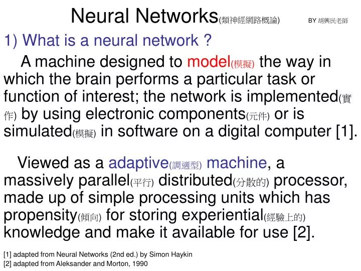
1. Neural Networks(類神經網路概論)BY 胡興民老師 1) What is a neural network ? A machine designed to model(模擬)the way in which the brain performs a particular task or function of interest; the network is implemented(實作) by using electronic components(元件) or is simulated(模擬) in software on a digital computer [1]. Viewed as a adaptive(調適型) machine, a massively parallel(平行) distributed(分散的) processor, made up of simple processing units which has propensity(傾向) for storing experiential(經驗上的) knowledge and make it available for use [2]. [1] adapted from Neural Networks (2nd ed.) by Simon Haykin [2] adapted from Aleksander and Morton, 1990

2. 2) significance(重要意義) for a neural network the ability tolearn from its environment(環境) and to improve its performance(性能) through learning. Learning is a process by which the free parameters(參數) of a neural network are adapted through a process of stimulationby environment [3]. The type of learning is determined(決定) by the manner in which the parameter changestake place(參數發生改變的方式). [3] adapted from Mendel and McClaren, 1970

3. 3) Five basic learning rules error-correction(錯誤更正式學習) learning (rooted in optimum filtering)(植基於最佳化過濾) memory-based(記憶型學習) learning (memorizing the training data explicitly(清楚地記住)) Hebbian learning, competitive(競爭型) learning (these two are inspired(啟發) by neurobiological(生物神經學上的) considerations) Boltzmann learning (based on statistical(統計學 上的) mechanics(機制))

4. Multilayer feedforward network (前饋式多層網路) Input vector Output neuron k One or more layers of hidden neurons yk(n) dk(n) X(n) Σ ﹣ ﹢ ek(n) Block diagram of a neural network, highlighting the only neuron (神經元) in the output layer

5. yk(n) is compared to a desired response or targetoutput,dk(n). Consequently, an error signal, ek(n), is produced. ek(n) = dk(n) ﹣yk(n) The error signal actuates adjustments(啟動調整) to the synaptic weights(神經腱強度) to make the output signal come closer to the desired response in a step-by-step manner. The objective is achieved by minimizing a cost functionor index of performance,ξ(n), and is the instantaneous value(即時值) of theerror energy: ξ(n) = ½ [ek(n)] 2 The adjustments are continued until the system reaches a steady state. Minimization of theξ(n) is referred to as the delta rule or Widrow-Hoff rule.

6. wk1(n) x1(n) x2(n) xj(n) xm(n) wk2(n) φ(‧) dk(n) X(n) -1 … wkj(n) … vk(n) yk(n) ek(n) … wkm(n) … Signal-flow graph of output neuron

7. Let wkj(n) denote the value of synaptic weight of neuron k excited(激發) by element xj(n) of the signal vector X(n) at time step n. The adjustment Δwkj(n) is defined by Δwkj(n) = ηek(n) xj(n) where η is a positive constant that determines the rate of learning as we proceed from one step in the learning process to another. The updated value of synaptic weight wkj is determined by wkj(n+1) = wkj(n) +Δwkj(n)

8. 5) memory-based learning There are correctly classified(正確分類的) input-output examples:｛(xi, di)｝, i = 1, …, N where xi is an input vector and di denotes(表示) the corresponding(相對應的) desired response. When classification of a test vector xtest (not seen before) is required, the algorithm responds by retrieving(回去擷取) and analyzing the training data in a “local neighborhood” of xtest .

9. Local neighborhood is defined as the training example that lies in(位於) the immediate(最近的近鄰) neighborhood of xtest (e.g. the network employs thenearest neighbor rule). For example, xN’ ∈｛x1, x2 , …, xN｝ is said to the nearest neighbor of xtest if mini d(xi, xtest) = d(xN’, xtest), i = 1, 2, …, N where d(xi, xtest) is the Euclidean distance between the vectors xi and xtest . The class associated with the minimum distance, that is, vector xN’, is reported as the classification of xtest .

10. A variant(類似方法) is the k-nearest neighbor classifier, which proceeds as follows: Identify(辨認出) the k classified patterns that lie nearest to the xtest for some integer k. assign xtest to the class (hypothesis) that is most frequently represented(代表) in the k nearest neighbor to xtest (i.e., use a majority vote(多數決) to make the classification and to discriminate(區分出) against the outlier(s)(外來者), as illustrated in the following figure for k = 3).

11. The red marks include two pointspertaining to (屬於) class 1 and an outlier from class 0. The point d corresponds to the test vector xtest . With k = 3, the k-nearest neighbor classifier assigns class 1 to xtest even though it lies closest to the outlier. 0 0 0 0 0 0 0 00 0 0 0 1 1 0 0 0d 0 1 1 1 11 1 1 1 1 1 11 1 1 1

12. 6) Hebbian learning the original Hebb rule: If two neurons on either side of a synapse (connection) are activated simultaneously(即刻地) (i.e., synchronously(同步地)), then the strength of that synapse is selectively increased. (ii) If two neurons on either side of a synapse are activated asynchronously(非同步地), then that synapse is selectively weakened(弱化) or eliminated(摘除) [4]. [4] Stent, 1973; Changeux and Danchin, 1976

13. xj(n), yk(n) denote presynaptic and postsynaptic signals respectively(各自地) at time step n, then the adjustment(Hebb’s hypothesis) is expressed by Δwkj(n) = ηyk(n) xj(n) The correlational(關連) nature of a Hebbian synapse is sometimes referred to as the activity product ruleas is shown in the top curve of the following figure, with the change Δwkj plotted verse the output signal (postsynaptic activity) yk.

14. Δwkj Hebb’s hypothesis Illustration of Hebb’s hypothesis and the covariance hypothesis Slope = ηxj slope = η(xj – Mx) Covariance hypothesis (共變異假說) 0 -η(xj - Mx)My postsynaptic activity, yk balance point Max. depression point

15. Covariance hypothesis [5]: xj(n), yk (n) are replaced by xj - Mx , yk - My respectively, where Mx /My denote the time-averaged value of xj/yk . Hence, theadjustment is described by Δwkj = η(xj - Mx)( yk - My) The average values x, y constitute thresholds(閥值), which determine the sign(跡象) of synaptic modification. [5] Sejnowski, 1977

16. 7) competitive learning The output neurons of a neural network competeamong themselves to become active (fired). Based on Hebbian learning several output neurons may be active simultaneously, while in competitive learning only a single output neuron is active at any one time.

17. Architectural graph of a simple competitive learning network with feedforward connections, and lateral connections(橫向腱值) among the neurons. layer of source nodes Single layer of output neurons x1 x2 x3 x4

18. Output signals yk of winning neuron k is set to one; the y of all losing neurons are set to zero. That is, yk = 1 if vk＞vj for all j, j≠k; yk = 0, otherwise where the induced local field(活化濳能) vk represents the combined action of all the forward and feedback inputs to neuron k. Suppose each neuron is allotted(配給) a fixed amount (i.e., positive) of synaptic weight, which is distributed among its input nodes; that is, Σj wkj = 1 for all k (j = 1, …, N) The change Δwkj applied to(作用於) wkj is defined by Δwkj = η(xj - wkj ) if neuron k wins the competition; Δwkj = 0 if k losing

19. x o o o o x o o o o o o x x o o o o o o o x o o o o o o o o o x (a) (b) Geometric interpretation(解讀) of the competitive learning process [6]. The o represents the input vectors, and the x the synaptic weight vectors of three output neurons. (a) representing initial state of the network (b) final state. (It is assumed(假設) that all neurons in the network are constrained(受限) to have the same Euclidean length, i.e. norm, as shown byΣj wkj2 = 1 , for all k (j = 1, …, N). [6] Rumelhart and Zipser, 1985

20. 8) boltzmann learning A recurrent (循環的) structure, and operating in a binary manner since they are either in an “on” state denoted by +1 or in an “off” state (-1). An energy function, E, is shown by E = -½ΣjΣk wkjxkxj (j≠k) where xj : state of neuron j, and j≠k meaning: none of the neurons has self-feedback. By choosing xk at random(隨機地) in the learning process, then flipping to(切換成) -xk at some pseudotemperature(類溫度) T with probability P(xk→ -xk) = [1 + exp(-ΔEk / T )]-1 where ΔEk : energy change resulting from such a flip. If applied repeatedly, the machine will reach thermal equilibrium.(熱平衡)

21. ρkj+ denote the correlation between the states of neuros j and k, with the network in its clamped condition1, whereas ρkj− denotes the correlation in free-running condition2. The change Δwkj is defined by [7] Δwkj = η(ρkj+ − ρkj− ), j≠k where both ρkj+ and ρkj− range in value from -1 to +1. Rk 1:Neurons providing an interface between the network and the environment are called visible. Visible neurons are all clamped(跼限於) onto specific states, whereas hidden neurons always operate freely. Rk 2: All neurons (visible and hidden) are allowed to operate freely in free-running condition. [7] Hinton and Sejnowski, 1986

22. vector describing state of the environment block diagram of supervised learning (監督式學習) desired response environment teacher + actual response Learning system Σ _ error signal 9) supervised learning (learning with a teacher)

23. Teacher has the knowledge of environment, with that knowledge being represented by a set of input-output examples. The environment is, however, unknown to the network of interest. The learning process takes place under the tutelage(監 護) of a teacher. The adjustment is carried out iteratively(疊代地執行) in a step-by-step fashion(方式)with the aim of eventually making the network emulate(盡量模仿) the teacher.

24. 10) Learning without a teacher No labeled(標明配對的) examples of the function are to be learned by the network, and two subdivision are identified: (i) reinforcement learning/ neuro- dynamic programming (ii) unsupervised learning. (i) reinforcement learning The learning of an input-output mapping is performed through continued interaction with the environment in order to minimize a scalar index of performance.

25. primary reinforcement state (input) vector environment critic heuristic reinforcement(啟發式的自行發展出補強) learning system action

26. (ii) unsupervised/self-organized learning(自組織 式學習) No external teacher or critic; rather, provision(預備) is made for a task-independent measure of the quality of representation that the network is required to learn, and the free parameters of the network are optimized with respect to(以該手段) that measure. Once the network tuned to(校準到) the statistical regularities of the input data, it develops the ability to form internal representations for encoding features(把特徵 編碼) and thereby to create new classes automatically.

27. vector describing state of the environment block diagram of unsupervised learning (非監督式學習) environment learning system

28. 11) learning tasks The choice of a particular learning algorithm is Influenced(影響) by the learning task. (i) pattern association(圖訊聯想) takes one of two forms: Autoassociation(自聯想) or heteroassociation (異聯想) . In autoassociation, a network is required to store a set of patterns (vectors) by repeatedly presenting (呈現) them to the network. The network is subsequently presented a partial description or distorted (noisy) version of an original pattern stored in it, and the task is to retrieve (recall) that particular pattern.

29. Heteroassociation differs from autoassociation in that an arbitrary set of input patterns is paired with another arbitrary set of output patterns. Autoassociation involves the use of unsupervised learning, whereas the type of learning involved in heteroassociation is supervised.

30. output vector y • Input vector x Pattern association (The key pattern xk acts as a stimulus(激勵源) that not only determines the storage location of memorized pattern yk, but also holds the key (即: 位址) for its retrieval.) input-output relation of pattern association

31. 1 2 r Unsupervised networked for feature extraction Supervised network for classification … (a) ․ Feature extraction ․x y․ classification m-dimensional observation space q- dimensional feature space (b) r- dimensional decision space Illustration of the approach to pattern classification (The network may take either forms.) (ii) pattern recognition: defined as the process whereby a receivedpattern/signal is assigned to one of a prescribed number of classes (categories). …

32. Associative memory(聯想記憶體) • 12) An associative memory offers the following • characteristics(特徵): • ․The memory is ditributed. • ․Information is stored in memory by setting up(建構) a • spatial pattern(空間圖訊) of neural activities. • ․Information contained in a stimulus(激勵源) not only • determines its storage location but also an address • for its retrival(再次被取用) • ․There may be interactions(互動) and so, there is • distinct(確切的) possibility to make errors during the • recall(回憶) process.

33. The memory is said to perform a distributed mapping (映射) that transforms(轉換) an activity pattern (圖訊訊息) in the input space into another activity pattern in the output space, as illustrated in the diagram. Yk1 Yk2 . . Ykm 1 2 . . m Xk1 Xk2 . . Xkm 1 2 . . m Input layer synaptic output layer of neurons junctions of neurons input layer output layer of source nodes of neurons (a) Associative M. model (b) associativeM. model using component of a nervous system artificial neurons

34. Xk1 Xk2 . . Xkm Wi1(k) Wi2(k) Wim(k) Yki The assumption: each neuron acts as a linear combiner, depicting in the following graph. An activity pattern xk , yk occurring in the input, output layer simultaneously, respectively is written in their expanded forms as: Xk=[xk1 , xk2 , …, xkm]T Yk=[yk1 , yk2 , …, ykm]T Signal-flow graph model of a linear neuron labeled i. . .

35. The association of vector Xk with memorized vector Yk is described in matrix form as: Yk=W(k) Xk , k=1,2, …,q where W(k) is determined by the input-output pair (Xk , Yk). A detailed description is given by yki= wij(k)xkj ,i=1,2, …, m Using matrix notation, yki is expressed in the equivalent form yki=[wi1(k), wi2(k), …, wim(k)] i=1,2, …, m

37. The individual presentations of the q pairs of associated patterns Xk→Yk , k=1,2, …, q produce corresponding values of the individual matrix, namely W(1), W(2), …, W(q). We define an m-by-m memory matrix that describes the summation of the weight matrices as follows: M= W(k) The matrix M defines the overall connectivity between the input and output layers of the associative memory. In effect, it also represents the total experience gained By the memory and can be reconstructed as a recursion shown by Mk=Mk-1+W(k) , k=1,2, …, q …(A)

38. where the initialvalueM0 is zero (i.e., the synaptic weights in the memory are all initially zero), and the final valueMq is identically equal to M. When W(k) is added to Mk-1, the increment W(k) loses its distinct identy among the mixture of contributions that form Mk , whereas information about the stimuli maynot have lost. Note: As the number q increases, the influence of a new pattern on the memory as a whole is progressively reduced.

39. Suppose the associative memory has learned M, we may postulate , denoting an estimate of M in terms of these patterns as [1]: = ykxkT …..(B) ykxkT represents the outer product of the xk and yk , and is an estimate of the W(k) that maps the output pattern yk onto the input pattern xk . xkj is the output of source node j in the input layer, and yki is the output of neuron i in the output layer. In the context of wij(k) for the kth association, source node j acts as a presynaptic node and neuron i acts as a postsynaptic node. [1] Anderson,1972, 1983; Cooper, 1970]:

40. The ‘local’ learning process in eq.(B) may be viewed as a generalization of Hebb’s postulate of learning. An associative memory so designed is called a correlation matrix memory. Correlation is the basis of learning, association, pattern recognition, and memory recall [2]. Eq.(B) may be reformulated: = YXt ……. (C) where X =[x1,x2, …, xq], called the key matrix, and Y=[y1, y2, …, yq], called the memorized matrix. [2] Eggermont, 1990

41. Eq.(C) may be reconstructed as a recursion and is depicted as follows: k=1,2, …, q ….(D) Comparing eq.(A) and (D), we see represents an estimate of the W(k). yk Z-1I X X

42. recall • The problem posed by an associative memory is the address and recall of patterns stored in memory. Let xj be picked at random and reapplied as stimuli to the memory, yielding the response y = xj …(E) Substituting eq.(B) in (E), we get y= yk xj = (xj)yk =( xj)yj + ( xj)yk =yj + ( xj)yk = yj + vj …(F)

43. yj of eq.(F) represents the “desired” response; It may be viewed as the “signal” component of the actual response y. vj is a “noise vector” that is responsible for making errors on recall. Let x1,x2, …, xq be normalized to have unit energy; i.e., Ek= = xk =1, k=1,2, …, q ∵ ∴ cos(xk,xj)= = xj ⇒ cos(xk,xj)=0, k≠j, if xk and xj are orthogonal. ⇒ vj= =0; i.e., in such a case, y=yj

44. ⇒ The memory associates perfectly if the key vectors form an orthogonal set; that is, if they satisfy the conditions: xj= Another question: What is the limit on the storage capacity of the associative memory? The answer lies in the rank (say r) of memory matrix Suppose a rectangular matrix has dimensions l-by-m, we then have r ≤ min(l,m). In the case of a correlation memory, is an m-by-m matrix. ⇒ r ≤ m ⇒ the number of patterns can never exceed the input space dimensionality.

45. What if the key patterns are neither orthogonal nor highly separated ? ⇒ a correlation matrix memory may get confused and make errors. • First, define the community of a set of patterns as the lower bound on the inner products xj. • Second, be further assumed that xj ≥λ, k≠j Ifλis large enough, the memory may fail to distinguish the response y from that of any other key pattern.

46. Say, xj=x0+ v ,where v is a stochastic vector. It is likely the memory will recognize x0 and associate with it a vector y0rather than any of the actual pattern pairs used to trained it. ⇒ x0 and y0 denote a pair of patterns never seen before. 兩題程式(MATLAB)練習(解析在隨後的slides): (1) 以 unsupervised方式, 將(0, 0), (0,1), (1,0), (1,1) 分成兩類, 即AND邏輯運算; Note: 一開始給定weight值, bias值; 並注意 完成分類後的weight值, bias值 (2) 將題(1)之輸入分成兩類, 但作OR邏輯運算且為supervised設計; Note:一開始未設定weight值, bias值 (即, 皆零值; 注意程式中的測試 !); 查看完成分類後的weight值, bias值; 請自行更改程式中 epoch值, 注意性能曲線變化及最後的weight值, bias值

47. close all;clear;clc; % 題(1): AND運算, unsupervised設計 % • net=newp([-2 2;-2 2],1); • net.IW{1,1}=[2 2]; • net.b{1}=[-3]; • % input vectors % • p1=[0;0]; • a1=sim(net,p1) • p2=[0;1]; • a2=sim(net,p2) • % a sequence of two input vectors % • p3={[0;0] [0;1]}; • a3=sim(net,p3) • % a sequence of four input vectors % • p4={[0;0] [0;1] [1;0] [1;1]}; • % simulated output and final wt./bias % • a4=sim(net,p4) • net.IW{1,1} • net.b{1} • % boundary / weight % • xx=-.5:.1:2; • yy=-net.b{1}/2-xx; • x2=0:.1:1.2; • y2=x2; • plot(xx,yy,0,0,'o',0,1,'o',1,0,'o',1,1,'x',x2,y2); • legend('boundary') • gtext('W')

48. close all;clear;clc; % 題(2): OR運算, supervised 設計; 並請更改 epoch值 % • net=newp([-2 2;-2 2],1); • testp=[1 1 1 1]; • net.IW{1,1} • net.b{1} • while testp ~= [0 0 0 0] • net.trainparam.epochs=4; • p=[[0;0] [0;1] [1;0] [1;1]]; • t=[0 1 1 1]; • net=train(net,p,t); • % the new weights and bias are % • net.IW{1,1} • net.b{1} • % simulate the trained network for each of the inputs % • a = sim(net,p) • % The errors for the various inputs are % • error = [a(1)-t(1) a(2)-t(2) a(3)-t(3) a(4)-t(4)] • testp=error; • end • xx=-1:.1:2; • yy=-net.b{1}-xx; • x2=xx-.2;y2=yy-.2; • x3=0:.01:.7; • y3=x3; • plot(x2,y2,0,0,'o',0,1,'x',1,0,'x',1,1,'x',x3,y3,'->') • legend('boundary') • gtext('weight')