Download
1 / 15
150 likes | 269 Views
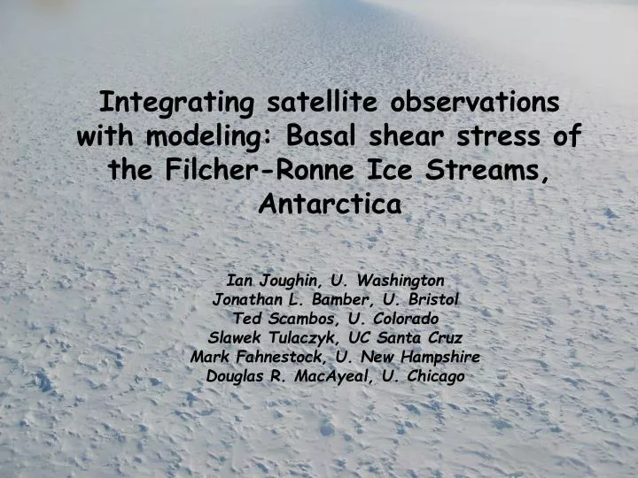
Integrating satellite observations with modeling: Basal shear stress of the Filcher-Ronne Ice Streams, Antarctica. Ian Joughin, U. Washington Jonathan L. Bamber, U. Bristol Ted Scambos, U. Colorado Slawek Tulaczyk, UC Santa Cruz Mark Fahnestock, U. New Hampshire

E N D
Integrating satellite observations with modeling: Basal shear stress of the Filcher-Ronne Ice Streams, Antarctica Ian Joughin, U. Washington Jonathan L. Bamber, U. Bristol Ted Scambos, U. Colorado Slawek Tulaczyk, UC Santa Cruz Mark Fahnestock, U. New Hampshire Douglas R. MacAyeal, U. Chicago
Filchner-Ronne Ice Streams Altimeter (Davis et al, 2005) and mass flux (Joughin and Bamber, 2005) estimates show this region is thickening.
Ross Ice Streams flow over a weak bed: Low profile ice sheet (ice stream flow). Variable ice flow. Much of the East Antarctic Ice Sheet flows over a strong bed: Typical concave down ice sheet profile (sheet flow). Greater stability. Bed Shear Stress
Filchner-Ronne Ice Streams • Several long ice streams flowing deep into the interior. • Large departures in several drainages from a “typical” ice sheet profile [Vaughan and Bamber, 1998]. • Bed properties determined at only a few locations with seismic surveys (Rutford and Evans).
zb zs V tb Control Method Inversion Procedure [MacAyeal, 1992] Control Method Inversions for Basal Shear Stress • Inversions are robust with respect to errors in velocity and bed topography. • Inversions are sensitive to surface elevation noise.
Driving Stress MOA – MODIS Mosaic of Antarctica
td = 43 kPa tb = 14 kPa td = 20 kPa tb = 6 kPa Recovery Ice Stream H = 786 m W = 50 km V = 244 m/yr
Recovery Ice Stream (cont.) • Flux through main trunk ~9 Gtons/yr. • Flux at grounding line 35 Gtons/yr. • This section drains ~80-90% of the catchment • 28 to 32 Gtons/yr. • Velocity and width well known • Thickness wrong by a factor of 3.2-3.6. • Almost no thickness data for this region. • The ice stream may flow through a trough that lies ~1400-1800 m below sea level.
Recovery Ice Stream (cont.) • Inversions with increased ice thickness yield • tb=18 • td=63 kPa. • Combination of a weak bed and thick ice in trough should have a major influence on this sector of the ice sheet.
td = 22 kPa tb = 10 kPa td = 45 kPa tb = 12 kPa Foundation Ice Stream
td = 10 kPa tb = 4 kPa td = 26 kPa tb = 11 kPa Institute Ice Stream
td = 45 kPa tb = 6 kPa Rutford Ice Stream
td = 30 kPa tb = 7 kPa td = 29 kPa tb = 8 kPa td = 32 kPa tb = 8 kPa Evans Ice Stream
Summary • A weak bed (~4 to 20 kPa) underlies much of the FR ice streams. • Beds beneath the FR ice streams have more “sticky” spots (regions) than beneath Ross Ice Streams. • Sticky regions and thicker ice likely contribute to greater basal melt and perhaps greater stability. • There are several weak regions where basal shear stress is comparable to the Ross Ice Streams (consistent with seismic results). • There may be deep unmapped troughs beneath Recovery and other (??) areas, making it difficult to accurately model this sector of the ice sheet.


![[u] [u:] [ou]](https://cdn4.slideserve.com/8524074/slide1-dt.jpg)