Basic Statistics for Scientific Research

1. Basic Statistics for Scientific Research

2. Outline • Descriptive Statistics • Frequencies & percentages • Means & standard deviations • Inferential Statistics • Correlation • T-tests • Chi-square • Logistic Regression

3. Types of Statistics/Analyses Descriptive Statistics Describing a phenomena • Frequencies • Basic measurements Inferential Statistics • Hypothesis Testing • Correlation • Confidence Intervals • Significance Testing • Prediction How many? How much? BP, HR, BMI, IQ, etc. Inferences about a phenomena Proving or disproving theories Associations between phenomena If sample relates to the larger population E.g., Diet and health

4. Descriptive Statistics Descriptive statistics can be used to summarize and describe a single variable (aka, UNIvariate) • Frequencies (counts) & Percentages • Use with categorical (nominal) data • Levels, types, groupings, yes/no, Drug A vs. Drug B • Means & Standard Deviations • Use with continuous (interval/ratio) data • Height, weight, cholesterol, scores on a test

5. Frequencies & Percentages Look at the different ways we can display frequencies and percentages for this data: Pie chart Table AKA frequency distributions – good if more than 20 observations Good if more than 20 observations Bar chart

6. Distributions The distribution of scores or values can also be displayed using Box and Whiskers Plots and Histograms

7. Ordinal Level Data Frequencies and percentages can be computed for ordinal data • Examples: Likert Scales (Strongly Disagree to Strongly Agree); High School/Some College/College Graduate/Graduate School

8. Interval/Ratio Data We can compute frequencies and percentages for interval and ratio level data as well • Examples: Age, Temperature, Height, Weight, Many Clinical Serum Levels Distribution of Injury Severity Score in a population of patients

9. Interval/Ratio Distributions The distribution of interval/ratio data often forms a “bell shaped” curve. • Many phenomena in life are normally distributed (age, height, weight, IQ).

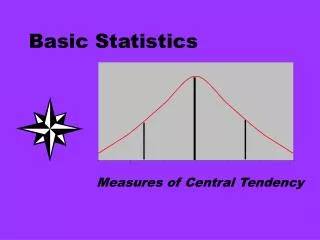
10. Interval & Ratio Data Measures of central tendency and measures of dispersion are often computed with interval/ratio data • Measures of Central Tendency (aka, the “Middle Point”) • Mean, Median, Mode • If your frequency distribution shows outliers, you might want to use the median instead of the mean • Measures of Dispersion (aka, How “spread out” the data are) • Variance, standard deviation, standard error of the mean • Describe how “spread out” a distribution of scores is • High numbers for variance and standard deviation may mean that scores are “all over the place” and do not necessarily fall close to the mean In research, means are usually presented along with standard deviations or standard errors.

11. INFERENTIAL STATISTICS Inferential statistics can be used to prove or disprove theories, determine associations between variables, and determine if findings are significant and whether or not we can generalize from our sample to the entire population The types of inferential statistics we will go over: • Correlation • T-tests/ANOVA • Chi-square • Logistic Regression

12. Type of Data & Analysis • Analysis of Categorical/Nominal Data • Correlation T-tests • T-tests • Analysis of Continuous Data • Chi-square • Logistic Regression

13. Correlation • When to use it? • When you want to know about the association or relationship between two continuous variables • Ex) food intake and weight; drug dosage and blood pressure; air temperature and metabolic rate, etc. • What does it tell you? • If a linear relationship exists between two variables, and how strong that relationship is • What do the results look like? • The correlation coefficient = Pearson’s r • Ranges from -1 to +1 • See next slide for examples of correlation results

14. Correlation Guide for interpreting strength of correlations: 0 – 0.25 = Little or no relationship 0.25 – 0.50 = Fair degree of relationship 0.50 - 0.75 = Moderate degree of relationship 0.75 – 1.0 = Strong relationship 1.0 = perfect correlation

15. Correlation • How do you interpret it? • If r is positive, high values of one variable are associated with high values of the other variable (both go in SAME direction - ↑↑ OR ↓↓) • Ex) Diastolic blood pressure tends to rise with age, thus the two variables are positively correlated • If r is negative, low values of one variable are associated with high values of the other variable (opposite direction - ↑↓ OR ↓ ↑) • Ex) Heart rate tends to be lower in persons who exercise frequently, the two variables correlate negatively • Correlation of 0 indicates NO linear relationship • How do you report it? • “Diastolic blood pressure was positively correlated with age (r = .75, p < . 05).” Tip: Correlation does NOT equal causation!!! Just because two variables are highly correlated, this does NOT mean that one CAUSES the other!!!

16. T-tests • When to use them? • Paired t-tests: When comparing the MEANS of a continuous variable in two non-independent samples (i.e., measurements on the same people before and after a treatment) • Ex) Is diet X effective in lowering serum cholesterol levels in a sample of 12 people? • Ex) Do patients who receive drug X have lower blood pressure after treatment then they did before treatment? • Independent samples t-tests: To compare the MEANS of a continuous variable in TWO independent samples (i.e., two different groups of people) • Ex) Do people with diabetes have the same Systolic Blood Pressure as people without diabetes? • Ex) Do patients who receive a new drug treatment have lower blood pressure than those who receive a placebo? Tip: if you have > 2 different groups, you use ANOVA, which compares the means of 3 or more groups

17. T-tests • What does a t-test tell you? • If there is a statistically significant difference between the mean score (or value) of two groups (either the same group of people before and after or two different groups of people) • What do the results look like? • Student’s t • How do you interpret it? • By looking at corresponding p-value • If p < .05, means are significantly different from each other • If p > 0.05, means are not significantly different from each other

18. How do you report t-testsresults? “As can be seen in Figure 1, children’s mean reading performance was significantly higher on the post-tests in all four grades, ( t = [insert from stats output], p < .05)” “As can be seen in Figure 1, specialty candidates had significantly higher scores on questions dealing with treatment than residency candidates (t = [insert t-value from stats output], p < .001).

19. Chi-square • When to use it? • When you want to know if there is an association between two categorical (nominal) variables (i.e., between an exposure and outcome) • Ex) Smoking (yes/no) and lung cancer (yes/no) • Ex) Obesity (yes/no) and diabetes (yes/no) • What does a chi-square test tell you? • If the observed frequencies of occurrence in each group are significantly different from expected frequencies (i.e., a difference of proportions)

20. Chi-square • What do the results look like? • Chi-square test statistics = X2 • How do you interpret it? • Usually, the higher the chi-square statistic, the greater likelihood the finding is significant, but you must look at the corresponding p-value to determine significance Tip: Chi square requires that there be 5 or more in each cell of a 2x2 table and 5 or more in 80% of cells in larger tables. No cells can have a zero count.

21. How do you report chi-square? “248 (56.4%) of women and 52 (16.6%) of men had abdominal obesity (Fig-2). The Chi square test shows that these differences are statistically significant (p<0.001).” “Distribution of obesity by gender showed that 171 (38.9%) and 75 (17%) of women were overweight and obese (Type I &II), respectively. Whilst 118 (37.3%) and 12 (3.8%) of men were overweight and obese (Type I & II), respectively (Table-II). The Chi square test shows that these differences are statistically significant (p<0.001).”

22. NORMAL DISTRIBUTION THE EXTENT OF THE ‘SPREAD’ OF DATA AROUND THE MEAN – MEASURED BY THE STANDARD DEVIATION MEAN CASES DISTRIBUTED SYMMETRICALLY ABOUT THE MEAN AREA BEYOND TWO STANDARD DEVIATIONS ABOVE THE MEAN

23. DESCRIBING DATA • In a normal distribution, mean and median are the same • If median and mean are different, indicates that the data are not normally distributed • The mode is of little if any practical use

24. BOXPLOT (BOX AND WHISKER PLOT) 97.5th Centile 75th Centile MEDIAN (50th centile) 25th Centile 2.5th Centile Inter-quartile range

25. Photo courtesy of Judy Davidson, DNP, RN

26. STANDARD DEVIATION – MEASURE OF THE SPREAD OF VALUES OF A SAMPLE AROUND THE MEAN THE SQUARE OF THE SD IS KNOWN AS THE VARIANCE • SD decreases as a function of: • smaller spread of values about the mean • larger number of values IN A NORMAL DISTRIBUTION, 95% OF THE VALUES WILL LIE WITHIN 2 SDs OF THE MEAN

27. Standard Deviation (σ) 99% 95%

28. STANDARD DEVIATION AND SAMPLE SIZE As sample size increases, so SD decreases n=150 n=50 n=10

29. How do we ESTIMATE Experimental Uncertainty due to unavoidable random errors?

30. Uncertainty in Multiple Measurements Since random errors are by nature, erratic, they are subject to the laws of probability or chance. A good way to estimate uncertainty is to take multiple measurements and use statistical methods to calculate the standard deviation. The uncertainty of a measurement can be reduced by repeating a measurement many times and taking the average. The individual measurements will be scattered around the average. The amount of spread of individual measurements around the average value is a measure of the uncertainty.

31. 62 63 64 65 66 67 68 Avr = 65.36 cm Larger spread or uncertainty Same average values Smaller spread or uncertainty The spread of the multiple measurements around an average value represents the uncertainty and is called the standard deviation, STD.

32. 2/3 (68%) of all the measurements fall within 1 STD 95% of all the measurements fall within 2 STDs 99% of all the measurements fall within 3 STDs The spread of the multiple measurements around an average value represents the uncertainty and is called the standard deviation, STD.

34. 68% confidence that another measurement would be within one STD of the average value. 95% confidence that another measurement would be within two STDs of the average value. 99% confidence that another measurement would be within three STDs of the average value. (between 5.1-8.9) (between 3.2-10.8) (between 1.3-12.7)

35. SKEWED DISTRIBUTION MEAN MEDIAN – 50% OF VALUES WILL LIE ON EITHER SIDE OF THE MEDIAN

36. DOES A VARIABLE FOLLOW A NORMAL DISTRIBUTION? • Important because parametric statistics assume normal distributions • Statistics packages can test normality • Distribution unlikely to be normal if: • Mean is very different from the median • Two SDs below the mean give an impossible answer (eg height <0 cm)

37. DISTRIBUTIONS: EXAMPLES

38. DISTRIBUTIONS AND STATISTICAL TESTS • Many common statistical tests rely on the variables being tested having a normal distribution • These are known as parametric tests • Where parametric tests cannot be used, other, non-parametric tests are applied which do not require normally distributed variables • Sometimes, a skewed distribution can be made sufficiently normal to apply parametric statistics by transforming the variable (by taking its square root, squaring it, taking its log, etc)

39. EXAMPLE: IQ Say that you have tested a sample of people on a validated IQ test The IQ test has been carefully standardized on a large sample to have a mean of 100 and an SD of 15 94 97 100 103 106

40. EXAMPLE: IQ Say you now administer the test to repeated samples of 25 people Expected random variation of these means equals the Standard Error 94 97 100 103 106

41. STANDARD DEVIATION vs STADARD ERROR • Standard Deviation is a measure of variability of scores in a particular sample • Standard Error of the Mean is an estimate of the variability of estimated population means taken from repeated samples of that population(in other words, it gives an estimate of the precision of the sample mean) See Douglas G. Altman and J. Martin Bland. Standard deviations and standard errors. BMJ 331 (7521):903, 2005.

42. EXAMPLE: IQ One sample of 25 people yields a mean IQ score of 107.5 What are the chances of obtaining an IQ of 107.5 or more in a sample of 25 people from the same population as that on which the test was standardized? 94 97 100 103 106

43. EXAMPLE: IQ How far out the sample IQ is in the population distribution is calculated as the area under the curve to the right of the sample mean: This ratio tells us how far out on the standard distribution we are – the higher the number, the further we are from the population mean 94 97 100 103 106

44. EXAMPLE: IQ Look up this figure (2.5) in a table of values of the normal distribution From the table, the area in the tail to the right of our sample mean is 0.006 (approximately 1 in 160) This means that there is a 1 in 160 chance that our sample mean came from the same population as the IQ test was standardized on 94 97 100 103 106

45. EXAMPLE: IQ This is commonly referred to as p=0.006 By convention, we accept as significantly different a sample mean which has a 1 in 20 chance (or less) of coming from the population in which the test was standardized (commonly referred to as p=0.05) Thus our sample had a significantly greater IQ than the reference population (p<0.05) 94 97 100 103 106

46. EXAMPLE: IQ If we move the sample mean (green) closer to the population mean (red), the area of the distribution to the right of the sample mean increases Even by inspection, the sample is more likely than our previous one to come from the original population 94 97 100 103 106

47. UNPAIRED OR INDEPENDENT-SAMPLE t-TEST: PRINCIPLE The two distributions are widely separated so their means clearly different The distributions overlap, so it is unclear whether the samples come from the same population In essence, the t-test gives a measure of the difference between the sample means in relation to the overall spread

48. UNPAIRED OF INDEPENDENT-SAMPLE t-TEST: PRINCIPLE With smaller sample sizes, SE increases, as does the overlap between the two curves, so value of t decreases

49. THE PREVIOUS IQ EXAMPLE • In the previous IQ example, we were assessing whether a particular sample was likely to have come from a particular population • If we had two samples (rather than sample plus population), we would compare these two samples using an independent-sample t-test

50. SUMMARY THUS FAR …