Lecture 2 Sparse matrix data structures, graphs , manipulation

1. 4th Gene Golub SIAM Summer School, 7/22 – 8/7, 2013, Shanghai Lecture 2Sparse matrix data structures, graphs, manipulation Xiaoye Sherry Li Lawrence Berkeley National Laboratory, USA xsli@lbl.gov crd-legacy.lbl.gov/~xiaoye/G2S3/

2. Lecture outline • PDE  discretization  sparse matrices • Sparse matrix storage formats • Sparse matrix-vector multiplication with various formats • Graphs associated with the sparse matrices • Distributed sparse matrix-vector multiplication

3. Solving partial differential equations • Hyperbolic problems (waves): • Sound wave (position, time) • Use explicit time-stepping: Combine nearest neighbors on grid • Solution at each point depends on neighbors at previous time • Elliptic (steady state) problems: • Electrostatic potential (position) • Everything depends on everything else, use implicit method • This means locality is harder to find than in hyperbolic problems • Canonical example is the Poisson equation • Parabolic (time-dependent) problems: • Temperature (position, time) • Involves an elliptic solve at each time-step 2u/x2 + 2u/y2 + 2u/z2 = f(x,y,z)

4. PDE discretization leads to sparse matrices • Poisson equation in 2D: • Finite difference discretization  stencil computation 5-point stencil

5. Matrix view Graph and “stencil” 4 -1 -1 -1 4 -1 -1 -1 4 -1 -1 4 -1 -1 -1 -1 4 -1 -1 -1 -1 4 -1 -1 4 -1 -1 -1 4 -1 -1 -1 4 -1 -1 4 -1 A = -1

6. Application 1: Burning plasma for fusion energy • ITER – a new fusion reactor being constructed in Cadarache, France • International collaboration: China, the European Union, India, Japan, Korea, Russia, and the United States • Study how to harness fusion, creating clean energy using nearly inexhaustible hydrogen as the fuel. ITER promises to produce 10 times as much energy than it uses — but that success hinges on accurately designing the device. • One major simulation goal is to predict microscopic MHD instabilities of burning plasma in ITER. This involves solving extended and nonlinear Magnetohydrodynamics equations.

7. Application 1: ITER modeling • US DOE SciDAC project (Scientific Discovery through Advanced Computing) • Center for Extended Magnetohydrodynamic Modeling (CEMM), PI: S. Jardin, PPPL • Develop simulation codes to predict microscopic MHD instabilities of burning magnetized plasma in a confinement device (e.g., tokamak used in ITER experiments). • Efficiency of the fusion configuration increases with the ratio of thermal and magnetic pressures, but the MHD instabilities are more likely with higher ratio. • Code suite includes M3D-C1, NIMROD R  Z • At each  = constant plane, scalar 2D data • is represented using 18 degree of freedom • quintic triangular finite elements Q18 • Coupling along toroidal direction (S. Jardin)

8. ITER modeling: 2-Fluid 3D MHD Equations The objective of the M3D-C1 project is to solve these equations as accurately as possible in 3D toroidal geometry with realistic B.C. and optimized for a low-β torus with a strong toroidal field.

9. Application 2: particle accelerator cavity design • USDOE SciDAC project • Community Petascale Project for Accelerator Science and Simulation (ComPASS), PI: P. Spentzouris, Fermilab • Development of a comprehensive computational infrastructure • for accelerator modeling and optimization • RF cavity: Maxwell equations in electromagnetic field • FEM in frequency domain leads to large sparse eigenvalue • problem; needs to solve shifted linear systems (L.-Q. Lee) RF unit in ILC E Closed Cavity Waveguide BC Waveguide BC Open Cavity M Waveguide BC

10. Nedelec-type finite-element discretization RF Cavity Eigenvalue Problem Find frequency and field vector of normal modes: “Maxwell’s Equations” E Closed Cavity M 10

11. Waveguide BC Waveguide BC Open Cavity Waveguide BC Cavity with Waveguide coupling for multiple waveguide modes • Vector wave equation with waveguide boundary conditions can be modeled by a non-linear complex eigenvalue problem where 11

12. Sparse: lots of zeros in matrix • fluid dynamics, structural mechanics, chemical process simulation, circuit simulation, electromagnetic fields, magneto-hydrodynamics, seismic-imaging, economic modeling, optimization, data analysis, statistics, . . . • Example: A of dimension 106, 10~100 nonzeros per row • Matlab: > spy(A) Boeing/msc00726 (structural eng.) • Mallya/lhr01 (chemical eng.)

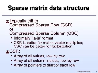
13. Sparse Storage Schemes • Assume arbitrary sparsitypattern … • Notation • N – dimension • NNZ – number of nonzeros • Obvious: • “triplets” format ({i, j, val}) is not sufficient . . . • Storage: 2*NNZ integers, NNZ reals • Not easy to randomly access one row or column • Linked list format provides flexibility, but not friendly on modern architectures . . . • Cannot call BLAS directly

14. 1 3 5 8 11 13 17 20 Nzval 1 a 2 b c d 3 e 4 f 5 g h i 6 j k l 7 (NNZ) colind 1 4 2 5 1 2 3 2 4 5 5 7 4 5 6 7 3 5 7 (NNZ) rowptr 1 3 5 8 11 13 17 20 (N+1) Compressed Row Storage (CRS) • Store nonzeros row by row contiguously • Example: N = 7, NNZ = 19 • 3 arrays: • Storage: NNZ reals, NNZ+N+1 integers

15. do i = 1, N . . . row i of A sum = 0.0 do j = rowptr(i), rowptr(i+1) – 1 sum = sum + nzval(j) * x(colind(j)) enddo y(i) = sum enddo 1 3 5 8 11 13 17 20 Nzval 1 a 2 b c d 3 e 4 f 5 g h i 6 j k l 7 (NNZ) colind 1 4 2 5 1 2 3 2 4 5 5 7 4 5 6 7 3 5 7 (NNZ) rowptr 1 3 5 8 11 13 17 20 (N+1) SpMV (y = Ax) with CRS • “dot product” • No locality for x • Vector length usually short • Memory-bound: 3 reads, 2 flops

16. nzval 1 c 2 d e 3 k a 4 h b f 5 i l 6 g j 7 (NNZ) rowind 1 3 2 3 4 3 7 1 4 6 2 4 5 6 7 6 5 6 7 (NNZ) colptr 1 3 6 8 11 16 17 20 (N+1) Compressed Column Storage (CCS) • Also known as Harwell-Boeing format • Store nonzeros columnwise contiguously • 3 arrays: • Storage: NNZ reals, NNZ+N+1 integers

17. nzval 1 c 2 d e 3 k a 4 h b f 5 i l 6 g j 7 (NNZ) rowind 1 3 2 3 4 3 7 1 4 6 2 4 5 6 7 6 5 6 7 (NNZ) colptr 1 3 6 8 11 16 17 20 (N+1) SpMV (y = Ax) with CCS • “SAXPY” • No locality for y • Vector length usually short • Memory-bound: 3 reads, 1 write, 2 flops y(i) = 0.0, i = 1…N do j = 1, N . . . column j of A t = x(j) do i = colptr(j), colptr(j+1) – 1 y(rowind(i)) = y(rowind(i)) + nzval(i) * t enddo enddo

18. Other Representations • “Templates for the Solution of Linear Systems: Building Blocks for Iterative Methods”, R. Barrett et al. (online) • ELLPACK, segmented-sum, etc. • “Block entry” formats (e.g., multiple degrees of freedom are associated with a single physical location) • Constant block size (BCRS) • Variable block sizes (VBCRS) • Skyline (or profile) storage (SKS) • Lower triangle stored row by row Upper triangle stored column by column • In each row (column), first nonzero defines a profile • All entries within the profile (some may be zero) are stored

19. SpMV optimization – mitigate memory access bottleneck BeBOP (Berkeley Benchmark and Optimization group): http://bebop.cs.berkeley.edu Software: OSKI / pOSKI – Optimized Sparse Kernel Interface • Matrix reordering: up to 4x over CSR • Register blocking: find dense blocks, pad zeros if needed, 2.1x over CSR • Cache blocking: 2.8x over CSR • Multiple vectors (SpMM): 7x over CSR • Variable block splitting • Symmetry: 2.8x over CSR • …

20. Graphs A graph G = (V, E) consists of a finite set V , called the vertex set and a finite, binary relation E on V , called the edge set. Three standard graph models • Undirected graph: The edges are unordered pair of vertices, i.e. • Directed graph: The edges are ordered pair of vertices, that is, (u, v) and (v, u) are two different edges • Bipartite graph: G = (U U V;E) consists of two disjoint vertex sets U and V such that for each edge An ordering or labelling of G = (V, E) having n vertices, i.e., |V|= n, is a mapping of V onto 1,2, …, n.

21. Graph for rectangular matrix • Bipartite graph Rows = vertex set U, columns = vertex set V each nonzero A(i,j) = an edge (ri,cj), ri in U and cj in V

22. Graphs for square, pattern nonsymmetric matrix • Bipartite graph as before • Directed graph: Rows / columns = vertex set V each nonzero A(i,j) = an ordered edge (vi, vj) directed vi vj

23. Graphs for square, pattern symmetric matrix • Bipartite graph as before • Undirected graph: Rows / columns = vertex set V each nonzero A(i,j) = an edge {vi, vj}

24. Parallel sparse matrix-vector multiply • y = A*x, where A is a sparse n x n matrix • Questions • which processors store • y[i], x[i], and A[i,j] • which processors compute • y[i] = (row i of A) * x … a sparse dot product • Partitioning • Partition index set {1,…,n} = N1  N2  … Np. • For all i in Nk, Processor k stores y[i], x[i], and row i of A • For all i in Nk, Processor k computes y[i] = (row i of A) * x • “owner computes”rule: Processor k compute y[i]s it owns P1 P2 P3 P4 X x x P1 P2 P3 P4 y i: [j1,v1], [j2,v2],… May need communication

25. 1 2 3 4 5 6 1 1 1 1 2 1 1 1 1 3 1 1 1 4 1 1 1 1 5 1 1 1 1 6 1 1 1 1 3 2 4 1 5 6 Graph partitioning and sparse matrices • A “good” partition of the graph has • equal (weighted) number of nodes in each part (load and storage balance). • minimum number of edges crossing between (minimize communication). • Reorder the rows/columns by putting all nodes in one partition together.

26. Matrix reordering via graph partitioning • “Ideal” matrix structure for parallelism: block diagonal • p (number of processors) blocks, can all be computed locally. • If no non-zeros outside these blocks, no communication needed • Can we reorder the rows/columns to get close to this? • Most nonzeros in diagonal blocks, very few outside P0 P1 P2 P3 P4 = * P0 P1 P2 P3 P4

27. Each process has a structure to store local part of A typedefstruct { intnnz_loc; // number of nonzeros in the local submatrix intm_loc; // number of rows local to this processor intfst_row; // global index of the first row void *nzval; // pointer to array of nonzero values, packed by row int*colind; // pointer to array of column indices of the nonzeros int*rowptr; // pointer to array of beginning of rows in nzval[]and colind[] } CRS_dist; Distributed Compressed Row Storage

28. Processor P0 data structure: nnz_loc = 5 m_loc = 2 fst_row = 0 // 0-based indexing nzval = { s, u, u, l, u } colind = { 0, 2, 4, 0, 1 } rowptr = { 0, 3, 5 } Processor P1 data structure: nnz_loc = 7 m_loc = 3 fst_row = 2 // 0-based indexing nzval = { l, p, e, u, l, l, r } colind = { 1, 2, 3, 4, 0, 1, 4 } rowptr = { 0, 2, 4, 7 } s u u P0 l u p l P1 e r l l Distributed Compressed Row Storage A is distributed on 2 cores: u

29. Sparse matrices in MATLAB • In matlab, “A = sparse()”, create a sparse matrix A • Type “help sparse”, or “doc sparse” • Storage: compressed column (CCS) • Operation on sparse (full) matrices returns sparse (full) matrix operation on mixed sparse & full matrices returns full matrix • Ordering: amd, symamd, symrcm, colamd • Factorization: lu, chol, qr, … • Utilities: spy

30. Summary • Many representations of sparse matrices • Depending on application/algorithm needs • Strong connection of sparse matrices and graphs • Many graph algorithms are applicable

31. References • Barrett, et al., “Templates for the solution of linear systems: Building Blocks for Iterative Methods, 2nd Edition”, SIAM, 1994 (book online) • Sparse BLAS standard: http://www.netlib.org/blas/blast-forum • BeBOP: http://bebop.cs.berkeley.edu/ • J.R. Gilbert, C. Moler, R. Schreiber, “Sparse Matrices In MATLAB: Design And Implementation”, SIAM J. Matrix Anal. Appl, 13, 333-356, 1992.

32. Exercises • Write a program that converts a matrix in CCS format to CRS format, see code in sparse_CCS/ directory • Write a program to compute y = A^T*x without forming A^T • A can be stored in your favorite compressed format • Write a SpMV code with ELLPACK representation • SpMV roofline model on your machine • Write an OpenMP program for SpMV • Run the MPI SpMV code in the Hands-On-Exercises/ directory

33. EXTRA SLIDES

34. ELLPACK • ELLPACK: software for solving elliptic problems [Purdue] • Force all rows to have the same length as the longest row, then columns are stored contiguously • 2 arrays: nzval(N,L) and colind(N,L), where L = max row length • N*L reals, N*L integers • Usually L << N

35. SpMV with ELLPACK • Neither “dot” nor “SAXPY” • Good for vector processor: long vector length (N) • Extra memory, flops for padded zeros, especially bad if row lengths vary a lot y(i) = 0.0, i = 1…N do j = 1, L do i = 1, N y(i) = y(i) + nzval(i, j) * x(colind(i, j)) enddo enddo

36. Segmented-Sum [Blelloch et al.] • Data structure is an augmented form of CRS, computational structure is similar to ELLPACK • Each row is treated as a segment in a long vector • Underlined elements denote the beginning of each segment (i.e., a row in A) • Dimension: S * L ~ NNZ, where L is chosen to approximate the hardware vector length

37. SpMV with Segmented-Sum • 2 arrays: nzval(S, L) and colind(S, L), where S*L ~ NNZ • NNZ reals, NNZ integers • SpMV is performed bottom-up, with each “row-sum” (dot) of Ax stored in the beginning of each segment • Similar to ELLPACK, but with more control logic in inner-loop • Good for vector processors do i = S, 1 do j = 1, L . . . enddo enddo