Download
1 / 55
560 likes | 833 Views
6.S093 Visual Recognition through Machine Learning Competition. Aditya Khosla and Joseph Lim. Image by kirkh.deviantart.com. Today’s class. Part 1: Introduction to deep learning What is deep learning? Why deep learning? Some common deep learning algorithms Part 2: Deep learning tutorial

E N D
6.S093 Visual Recognition through Machine Learning Competition AdityaKhosla and Joseph Lim Image by kirkh.deviantart.com
Today’s class • Part 1: Introduction to deep learning • What is deep learning? • Why deep learning? • Some common deep learning algorithms • Part 2: Deep learning tutorial • Please install Python++ now!
Slide credit • Many slides are taken/adapted from Andrew Ng’s
Typical goal of machine learning output input Label: “Motorcycle” Suggest tags Image search … ML images/video Speech recognition Music classification Speaker identification … ML audio Web search Anti-spam Machine translation … ML text
Typical goal of machine learning Feature engineering: most time consuming! output input Label: “Motorcycle” Suggest tags Image search … ML images/video Speech recognition Music classification Speaker identification … ML audio Web search Anti-spam Machine translation … ML text
Our goal in object classification “motorcycle” ML
But the camera sees this: Why is this hard? You see this:
Pixel-based representation pixel 1 Learning algorithm pixel 2 Input Motorbikes “Non”-Motorbikes Raw image pixel 2 pixel 1
Pixel-based representation pixel 1 Learning algorithm pixel 2 Input Motorbikes “Non”-Motorbikes Raw image pixel 2 pixel 1
Pixel-based representation pixel 1 Learning algorithm pixel 2 Input Motorbikes “Non”-Motorbikes Raw image pixel 2 pixel 1
What we want handlebars Feature representation Learning algorithm wheel E.g., Does it have Handlebars? Wheels? Input Motorbikes “Non”-Motorbikes Raw image Features pixel 2 Wheels Handlebars pixel 1
Some feature representations Spin image SIFT RIFT HoG GLOH Textons
Some feature representations Coming up with features is often difficult, time-consuming, and requires expert knowledge. Spin image SIFT RIFT HoG GLOH Textons
The brain: potential motivation for deep learning Auditory Cortex Auditory cortex learns to see! [Roe et al., 1992]
The brain adapts! Human echolocation (sonar) Seeing with your tongue Implanting a 3rd eye Haptic belt: Direction sense [BrainPort; Welsh & Blasch, 1997; Nagel et al., 2005; Constantine-Paton & Law, 2009]
Basic idea of deep learning • Also referred to as representation learning or unsupervised feature learning (with subtle distinctions) • Is there some way to extract meaningful features from data even without knowing the task to be performed? • Then, throw in some hierarchical ‘stuff’ to make it ‘deep’
Feature learning problem • Given a 14x14 image patch x, can represent it using 196 real numbers. • Problem: Can we find a learn a better feature vector to represent this? 255 98 93 87 89 91 48 …
First stage of visual processing: V1 V1 is the first stage of visual processing in the brain. Neurons in V1 typically modeled as edge detectors: Neuron #1 of visual cortex (model) Neuron #2 of visual cortex (model)
Learning sensor representations Sparse coding (Olshausen & Field,1996) Input: Images x(1), x(2), …, x(m)(each in Rn x n) Learn: Dictionary of bases f1, f2, …, fk(also Rn x n), so that each input x can be approximately decomposed as: xajfj s.t.aj’s are mostly zero (“sparse”) k j=1
Sparse coding illustration Natural Images Learned bases (f1 , …, f64): “Edges” »0.8 * + 0.3 * + 0.5 * Test example x»0.8 * f36+ 0.3 * f42+ 0.5 * f63 [a1, …, a64] = [0, 0, …, 0,0.8, 0, …, 0, 0.3, 0, …, 0, 0.5, 0] (feature representation)
0.6 *+ 0.8 *+ 0.4 * 15 28 37 1.3 *+ 0.9 *+ 0.3 * 5 18 29 Sparse coding illustration Represent as: [a15=0.6, a28=0.8, a37 = 0.4] Represent as: [a5=1.3, a18=0.9, a29 = 0.3] • Method “invents” edge detection • Automatically learns to represent an image in terms of the edges that appear in it. Gives a more succinct, higher-level representation than the raw pixels. • Quantitatively similar to primary visual cortex (area V1) in brain.
Going deep object models object parts (combination of edges) edges Training set: Aligned images of faces. pixels [Honglak Lee]
Why deep learning? Task: video activity recognition [Le, Zhou & Ng, 2011]
Audio Images Galaxy Video Text/NLP Multimodal (audio/video)
ImageNet classification: 22,000 classes … smoothhound, smoothhound shark, Mustelusmustelus American smooth dogfish, Musteluscanis Florida smoothhound, Mustelusnorrisi whitetipshark, reef whitetip shark, Triaenodonobseus Atlantic spiny dogfish, Squalusacanthias Pacific spiny dogfish, Squalussuckleyi hammerhead, hammerhead shark smooth hammerhead, Sphyrnazygaena smalleyehammerhead, Sphyrnatudes shovelhead, bonnethead, bonnet shark, Sphyrnatiburo angel shark, angelfish, Squatinasquatina, monkfish electric ray, crampfish, numbfish, torpedo smalltoothsawfish, Pristispectinatus guitarfish roughtailstingray, Dasyatiscentroura butterflyray eagle ray spotted eagle ray, spotted ray, Aetobatusnarinari cownoseray, cow-nosed ray, Rhinopterabonasus manta, manta ray, devilfish Atlantic manta, Manta birostris devil ray, Mobulahypostoma grey skate, gray skate, Raja batis little skate, Raja erinacea … Stingray Mantaray
ImageNet Classification: 14M images, 22k categories 0.005% 9.5% ? Random guess State-of-the-art (Weston, Bengio ‘11) Feature learning From raw pixels Le, et al., Building high-level features using large-scale unsupervised learning. ICML 2012
ImageNet Classification: 14M images, 22k categories 0.005% 9.5% 21.3% Random guess State-of-the-art (Weston, Bengio ‘11) Feature learning From raw pixels Le, et al., Building high-level features using large-scale unsupervised learning. ICML 2012
Some common deep architectures • Autoencoders • Deep belief networks (DBNs) • Convolutional variants • Sparse coding
Logistic regression Logistic regression has a learned parameter vector q. On input x, it outputs: where x1 x2 Draw a logistic regression unit as: x3 +1
Neural Network a1 String a lot of logistic units together. Example 3 layer network: a2 x1 a3 x2 x3 Layer 3 +1 +1 Layer 1 Layer 3
Neural Network Example 4 layer network with 2 output units: x1 x2 x3 +1 Layer 4 +1 +1 Layer 3 Layer 1 Layer 2
Training a neural network Given training set (x1, y1), (x2, y2), (x3, y3 ), …. Adjust parameters q (for every node) to make: (Use gradient descent. “Backpropagation” algorithm. Susceptible to local optima.)
Unsupervised feature learning with a neural network x1 x1 • Autoencoder. • Network is trained to output the input (learn identify function). • Trivial solution unless: • Constrain number of units in Layer 2 (learn compressed representation), or • Constrain Layer 2 to be sparse. x2 x2 x3 x3 a1 x4 x4 x5 x5 a2 +1 x6 x6 a3 Layer 2 Layer 3 +1 Layer 1
Unsupervised feature learning with a neural network x1 x1 x2 x2 a1 x3 x3 a2 x4 x4 a3 x5 x5 +1 x6 x6 Layer 2 Layer 3 +1 Layer 1
Unsupervised feature learning with a neural network x1 x2 a1 x3 a2 x4 a3 x5 +1 New representation for input. x6 Layer 2 +1 Layer 1
Unsupervised feature learning with a neural network x1 x2 a1 x3 a2 x4 a3 x5 +1 x6 Layer 2 +1 Layer 1
Unsupervised feature learning with a neural network x1 x2 a1 b1 x3 a2 b2 x4 a3 b3 x5 +1 +1 x6 Train parameters so that , subject to bi’s being sparse. +1
Unsupervised feature learning with a neural network x1 x2 a1 b1 x3 a2 b2 x4 a3 b3 x5 +1 +1 x6 Train parameters so that , subject to bi’s being sparse. +1
Unsupervised feature learning with a neural network x1 x2 a1 b1 x3 a2 b2 x4 a3 b3 x5 +1 +1 x6 Train parameters so that , subject to bi’s being sparse. +1
Unsupervised feature learning with a neural network x1 x2 a1 b1 x3 a2 b2 x4 a3 b3 x5 +1 +1 New representation for input. x6 +1
Unsupervised feature learning with a neural network x1 x2 a1 b1 x3 a2 b2 x4 a3 b3 x5 +1 +1 x6 +1
Unsupervised feature learning with a neural network x1 x2 a1 b1 c1 x3 a2 b2 c2 x4 a3 b3 c3 x5 +1 +1 +1 x6 +1
Unsupervised feature learning with a neural network x1 x2 a1 b1 c1 x3 a2 b2 c2 x4 a3 b3 c3 x5 New representation for input. +1 +1 +1 x6 +1 Use [c1, c3, c3] as representation to feed to learning algorithm.
Deep Belief Net Deep Belief Net (DBN) is another algorithm for learning a feature hierarchy. Building block: 2-layer graphical model (Restricted Boltzmann Machine). Can then learn additional layers one at a time.
Restricted Boltzmann machine (RBM) a1 a2 a3 Layer 2. [a1, a2, a3] (binary-valued) x2 x1 x3 x4 Input [x1, x2, x3, x4] MRF with joint distribution: Use Gibbs sampling for inference. Given observed inputs x, want maximum likelihood estimation:
Restricted Boltzmann machine (RBM) a1 a2 a3 Layer 2. [a1, a2, a3] (binary-valued) x2 x1 x3 x4 Input [x1, x2, x3, x4] Gradient ascent on log P(x) : [xiaj]obs from fixing x to observed value, and sampling a from P(a|x). [xiaj]prior from running Gibbs sampling to convergence. Adding sparsity constraint on ai’s usually improves results.
Deep Belief Network Similar to a sparse autoencoder in many ways. Stack RBMs on top of each other to get DBN. Layer 3. [b1, b2, b3] Layer 2. [a1, a2, a3] Input [x1, x2, x3, x4] Train with approximate maximum likelihood (often with sparsity constraint on ai’s):