Download

1 / 30
300 likes | 535 Views
Boosting. CMPUT 466/551 Principal Source: CMU. Boosting Idea. We have a weak classifier, i.e., it’s error rate is slightly better than 0.5. Boosting combines a lot of such weak learners to make a strong classifier (the error rate of which is much less than 0.5).

E N D
Boosting CMPUT 466/551 Principal Source: CMU
Boosting Idea We have a weak classifier, i.e., it’s error rate is slightly better than 0.5. Boosting combines a lot of such weak learners to make a strong classifier (the error rate of which is much less than 0.5)
Boosting: Combining Classifiers What is ‘weighted sample?’
Discrete Ada(ptive)boost Algorithm • Create weight distribution W(x) over N training points • Initialize W0(x) = 1/N for all x, step T=0 • At each iteration T : • Train weak classifier CT(x) on data using weights WT(x) • Get error rate εT . Set αT = log ((1 - εT )/εT ) • Calculate WT+1(xi ) = WT(xi ) ∙ exp[αT ∙ I(yi ≠ CT(xi ))] • Final classifier CFINAL(x) =sign [ ∑ αi Ci (x) ] • Assumes weak method CT can use weights WT(x) • If this is hard, we can sample using WT(x)
Real Adaboost Algorithm • Create weight distribution W(x) over N training points • Initialize W0(x) = 1/N for all x, step T=0 • At each iteration T : • Train weak classifier CT(x) on data using weights WT(x) • Obtain class probabilities pT(xi) for each data point xi • Set fT(x) = ½ log [ pT(xi)/(1- pT(xi)) ] • Calculate WT+1(xi ) = WT(xi ) ∙ exp[yi ∙fT(x)]for all xi • Final classifier CFINAL(x) =sign [ ∑ ft(x) ]
Performance of Boosting with Stumps Problem: Xj are standard Gaussian variables About 1000 positive and 1000 negative training examples 10,000 test observations Weak classifier is a “stump” i.e., a two-terminal node classification tree
AdaBoost is Special • The properties of the exponential loss function cause the AdaBoost algorithm to be simple. • AdaBoost’s closed form solution is in terms of minimized training set error on weighted data. • This simplicity is very special and not true for all loss functions!
Boosting: An Additive Model Consider the additive model: Can we minimize this cost function? N: number of training data points L: loss function b: basis functions This optimization is Non-convex and hard! Boosting takes a greedy approach
Boosting: Forward stagewisegreedy search Adding basis one by one
Boosting As Additive Model • Simple case: Squared-error loss • Forward stagewise modeling amounts to just fitting the residuals from previous iteration • Squared-error loss not robust for classification
Boosting As Additive Model • AdaBoost for Classification: • L(y, f (x)) = exp(-y ∙ f (x)) - the exponential loss function • Margin ≡ y ∙ f (x) Note that we use a property of the exponential loss function at this step. Many other functions (e.g. absolute loss) would start getting in the way…
Boosting As Additive Model First assume that β is constant, and minimize G:
Boosting As Additive Model First assume that β is constant, and minimize G: So if we choose G such that training error errmon the weighted data is minimized, that’s our optimal G.
Boosting As Additive Model Next, assume we have found this G, so given G, we next minimize β: Another property of the exponential loss function is that we get an especially simple derivative
Boosting: Practical Issues • When to stop? • Most improvement for first 5 to 10 classifiers • Significant gains up to 25 classifiers • Generalization error can continue to improveeven after training error is zero! • Methods: • Cross-validation • Discrete estimate of expected generalization error EG • How are bias and variance affected? • Variance usually decreases • Boosting can give reduction in both bias and variance
Boosting: Practical Issues • When can boosting have problems? • Not enough data • Really weak learner • Really strong learner • Very noisy data • Although this can be mitigated • e.g. detecting outliers, or regularization methods • Boosting can be used to detect noise • Look for very high weights
Features of Exponential Loss • Advantages • Leads to simple decomposition into observation weights + weak classifier • Smooth with gradually changing derivatives • Convex • Disadvantages • Incorrectly classified outliers may get weighted too heavily (exponentially increased weights), leading to over-sensitivity to noise
Squared Error Loss Explanation of Fig. 10.4:
Other Loss Functions For Classification • Logistic Loss • Very similar population minimizer to exponential • Similar behavior for positive margins, very different for negative margins • Logistic is more robust against outliers and misspecified data
Other Loss Functions For Classification • Hinge (SVM) • General Hinge (SVM) • These can give improved robustness or accuracy, but require more complex optimization methods • Boosting with exponential loss is linear optimization • SVM is quadratic optimization
Loss Functions for Regression • Squared-error Loss weights outliers very highly • More sensitive to noise, long-tailed error distributions • Absolute Loss • Huber Loss is hybrid:
Boosting and SVM • Boosting increases the margin “yf(x)” by additive stagewise optimization • SVM also maximizes the margin “yf(x)” • The difference is in the loss function– Adaboost uses exponential loss, while SVM uses “hinge loss” function • SVM is more robust to outliers than Adaboost • Boosting can turn base weak classifiers into a strong one, SVM itself is a strong classifier
Summary • Boosting combines weak learners to obtain a strong one • From the optimization perspective, boosting is a forward stage-wise minimization to maximize a classification/regression margin • It’s robustness depends on the choice of the Loss function • Boosting with trees is claimed to be “best off-the-self classification” algorithm • Boosting can overfit!