Download
1 / 20
250 likes | 560 Views
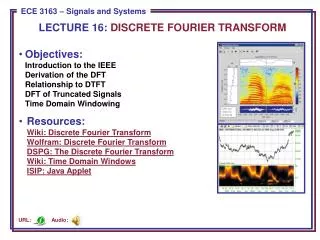
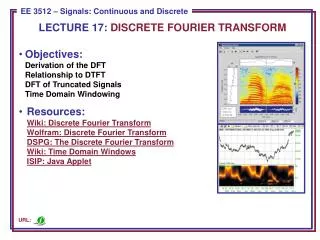
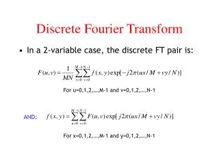
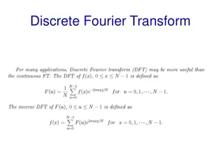
Discrete Fourier Transform. FFT and Its Applications.

E N D
FFT and Its Applications FFTSHIFT Shift zero-frequency component to the center of spectrum. For vectors, FFTSHIFT(X) swaps the left and right halves of X. For matrices, FFTSHIFT(X) swaps the first and third quadrants and the second and fourth quadrants. For N-D arrays, FFTSHIFT(X) swaps "half-spaces" of X along each dimension.
fftBox.m – Plot Fourier Spectrum • % • % Script file: fftBox.m • % Fourier Spectrum Plot of Box function • % • X1=linspace(0,1,17); • Y1=ones(1,length(X1)); • X2=linspace(1,16,241); • Y2=zeros(1,length(X2)); • X=[X1 X2]; Y=[Y1 Y2]; • W=abs(fftshift(fft(Y))); • subplot(2,1,1) • plot(X,Y,'r'); axis([0 16, 0,1.2]); title('Box function') • subplot(2,1,2) • plot(W,'b-'); • title('Fourier Spectrum of Box function')
Example of 2-D FFT Matlab Code • % Script file: fourier.m - 2D Fourier Transform • % Pictures on P.113 of Gonzalez, Woods, Eddins • m=128; n=128; • f=zeros(m,n); • f(56:71,48:79)=255; • F0=fft2(f); S0=abs(F0); • Fc=fftshift(fft2(f)); Sc=abs(Fc); • Fd=fft2(fftshift(f)); Sd=log(1+abs(Fc)); • subplot(2,2,1) • imshow(f,[]) • subplot(2,2,2) • imshow(S0,[]) • subplot(2,2,3) • imshow(Sc,[ ]) • subplot(2,2,4) • imshow(Sd,[ ])
Discrete Cosine Transform Partition an image into nonoverlapping 8 by 8 blocks, and apply a 2d DCT on each block to get DC and AC coefficients. Most of the high frequency coefficients become insignificant, only the DC term and some low frequency AC coefficients are significant. Fundamental for JPEG Image Compression
Discrete Cosine Transform (DCT) X: a block of 8x8 pixels A=Q8: 8x8 DCT matrix as shown above Y=AXAt
Matlab Code for 2d DCT • Q=xlsread('Qtable.xls','A2:H9'); • fin=fopen('block8x8.txt','r'); • fout=fopen('dctO.txt','w'); • fgetl(fin); X=fscanf(fin,'%f',[8,8]); fclose(fin); X=X'; • Y=dct2(X-128,[8,8]); • fprintf(fout,'DCT coefficients\n'); • for i=1:8 • for j=1:8 fprintf(fout,'%6.1f',Y(i,j)); end; fprintf(fout,'\n'); • end • Y=Y./Q; % Y=fix(Y+0.5*(Y>0)); • for i=1:8 • for j=1:8 • if (Y(i,j)>0) Y(i,j)=fix(Y(i,j)+0.5); else Y(i,j)=fix(Y(i,j)-0.5); end • end • end • fprintf(fout,'Quantized DCT coefficients\n'); • for i=1:8 • for j=1:8 fprintf(fout,'%4d',Y(i,j)); end; fprintf(fout,'\n'); • end • fclose(fout);
DCT-Based JPEG Conversion Input image write to file huffman encoding shift 128 DCT run-length encoding convert 2D matrix to 1D array round quantize with quantize matrix
Standard Quantization Table run-length encoding 產生一維結果: -26,-3,0,……,-1,-1,0,0,0,0……. 後皆為零,簡化可以減少資料儲存量
JPEG Decoding image result read compression file huffman decoding shift 128 IDCT run-length decoding quantize with quantize matrix convert 1D array to 2D matrix